In this workshop, we are using tsibble objects. They provide a data infrastructure for tidy temporal data with wrangling tools, adapting the tidy data principles.
In tsibble:
Index: time information about the observation
Measured variable(s): numbers of interest
Key variable(s): set of variables that define observational units over time
med_tsb |>fill_gaps(quantity_issued=0L) # we can fill it with zero
# A tsibble: 8,795 x 4 [1M]
# Key:       hub_id, product_id [133]
       date hub_id product_id quantity_issued
      <mth> <chr>  <chr>                <dbl>
 1 2017 Aug hub_1  product_1              721
 2 2017 Sep hub_1  product_1              795
 3 2017 Oct hub_1  product_1             1720
 4 2017 Nov hub_1  product_1              911
 5 2017 Dec hub_1  product_1              314
 6 2018 Jan hub_1  product_1             6913
 7 2018 Feb hub_1  product_1             2988
 8 2018 Mar hub_1  product_1             7120
 9 2018 Apr hub_1  product_1             3122
10 2018 May hub_1  product_1            11737
# ℹ 8,785 more rows
Check temporal gaps (implicit missing values)
Note: Since the main focus of this study is to provide foundational knowledge on forecasting, we will filter out time series with many missing values and then fill the remaining gaps using na.interp() function (Read more).
item_ids <- med_tsb |>count_gaps() |>group_by(hub_id, product_id) |>summarise(.n =max(.n), .groups ='drop') |>filter(.n >1) |>mutate(id =paste0(hub_id,'-',product_id)) |>pull(id) # filtering the item idsmed_tsb_filter <- med_tsb |>mutate(id =paste0(hub_id,'-',product_id)) |>group_by(hub_id, product_id) |>mutate(num_observations =n()) |>filter(!id %in% item_ids & num_observations >59) |># we have cold starts and discontinuations. fill_gaps(quantity_issued =1e-6, .full =TRUE) |># Replace NAs with a small valueselect(-id, -num_observations) |>mutate(quantity_issued =if_else(is.na(quantity_issued), exp( forecast::na.interp(ts(log(quantity_issued), frequency =12))), quantity_issued))
Data wrangaling using tsibble
We can use the filter() function to select rows.
med_tsb |>filter(hub_id =='hub_10')
# A tsibble: 417 x 4 [1M]
# Key:       hub_id, product_id [7]
       date hub_id product_id quantity_issued
      <mth> <chr>  <chr>                <dbl>
 1 2017 Jul hub_10 product_1              343
 2 2017 Aug hub_10 product_1               67
 3 2017 Sep hub_10 product_1              127
 4 2017 Oct hub_10 product_1              287
 5 2017 Nov hub_10 product_1              759
 6 2017 Dec hub_10 product_1              181
 7 2018 Jan hub_10 product_1             7015
 8 2018 Feb hub_10 product_1              840
 9 2018 Mar hub_10 product_1             4111
10 2018 Apr hub_10 product_1             1910
# ℹ 407 more rows
Data wrangaling using tsibble
We can use the select() function to select columns.
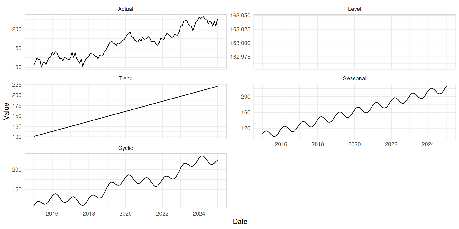
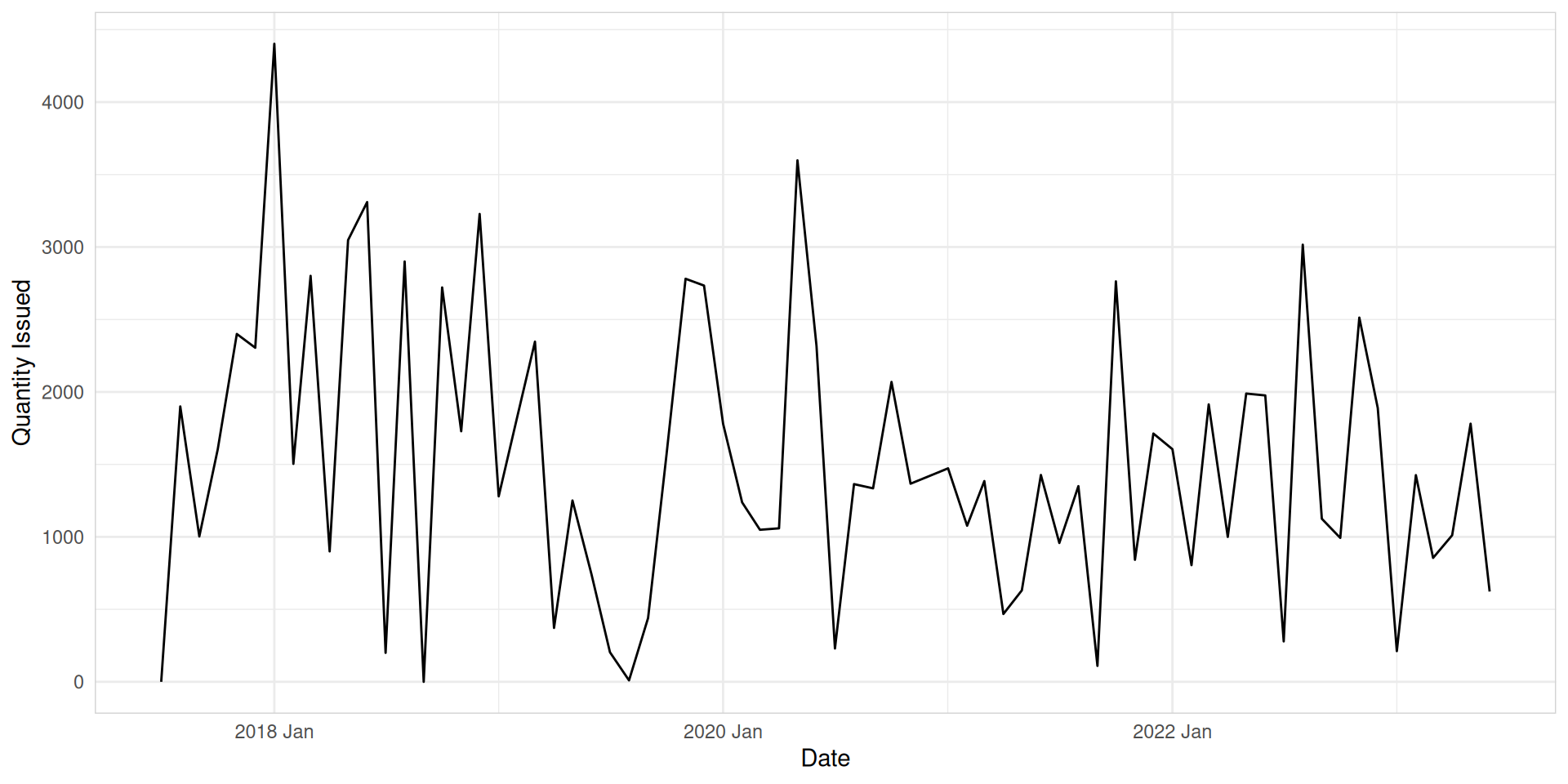
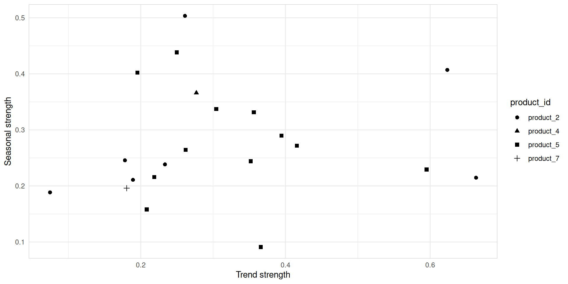
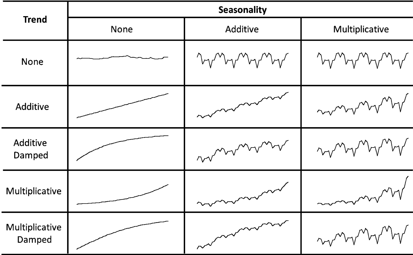
Level: The level of a time series describes the center of the series.
Trend: A trend describes predictable increases or decreases in the level of a series.
Seasonal: Seasonality is a consistent pattern that repeats over a fixed cycle. pattern exists when a series is influenced by seasonal factors (e.g., the quarter of the year, the month, or day of the week).
Cyclic: A pattern exists when data exhibit rises and falls that are not of fixed period (duration usually of at least 2 years).
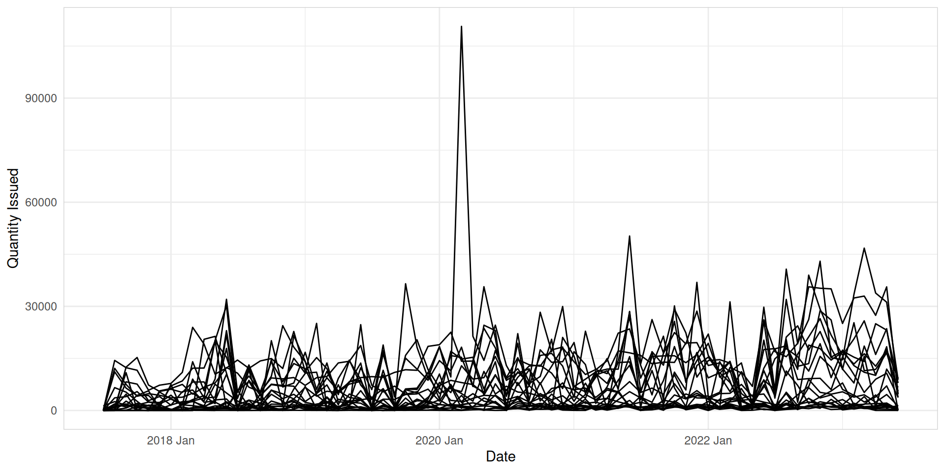
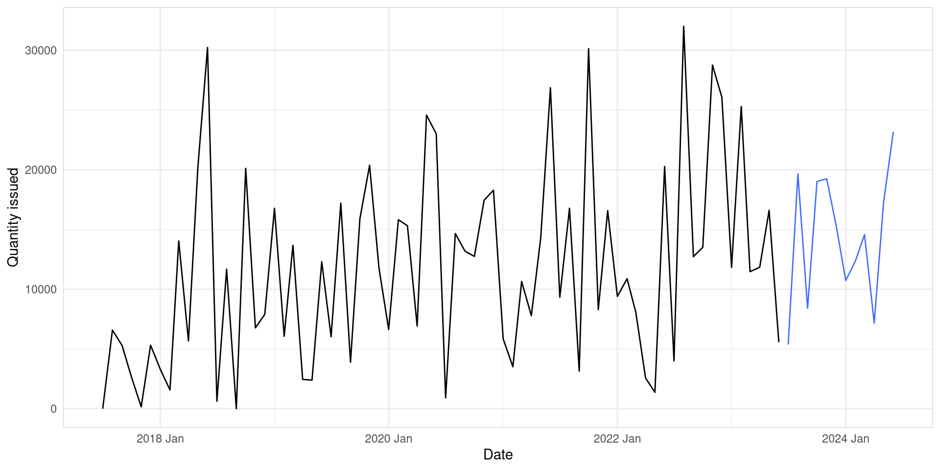
med_tsb_filter |>mutate(id =paste0(hub_id, product_id)) |>ggplot(aes(x = date, y = quantity_issued, group = id)) +geom_line() +labs(x ="Date",y ="Quantity Issued" ) +theme_minimal() +theme(legend.position ="none",panel.border =element_rect(color ="lightgrey", fill =NA))
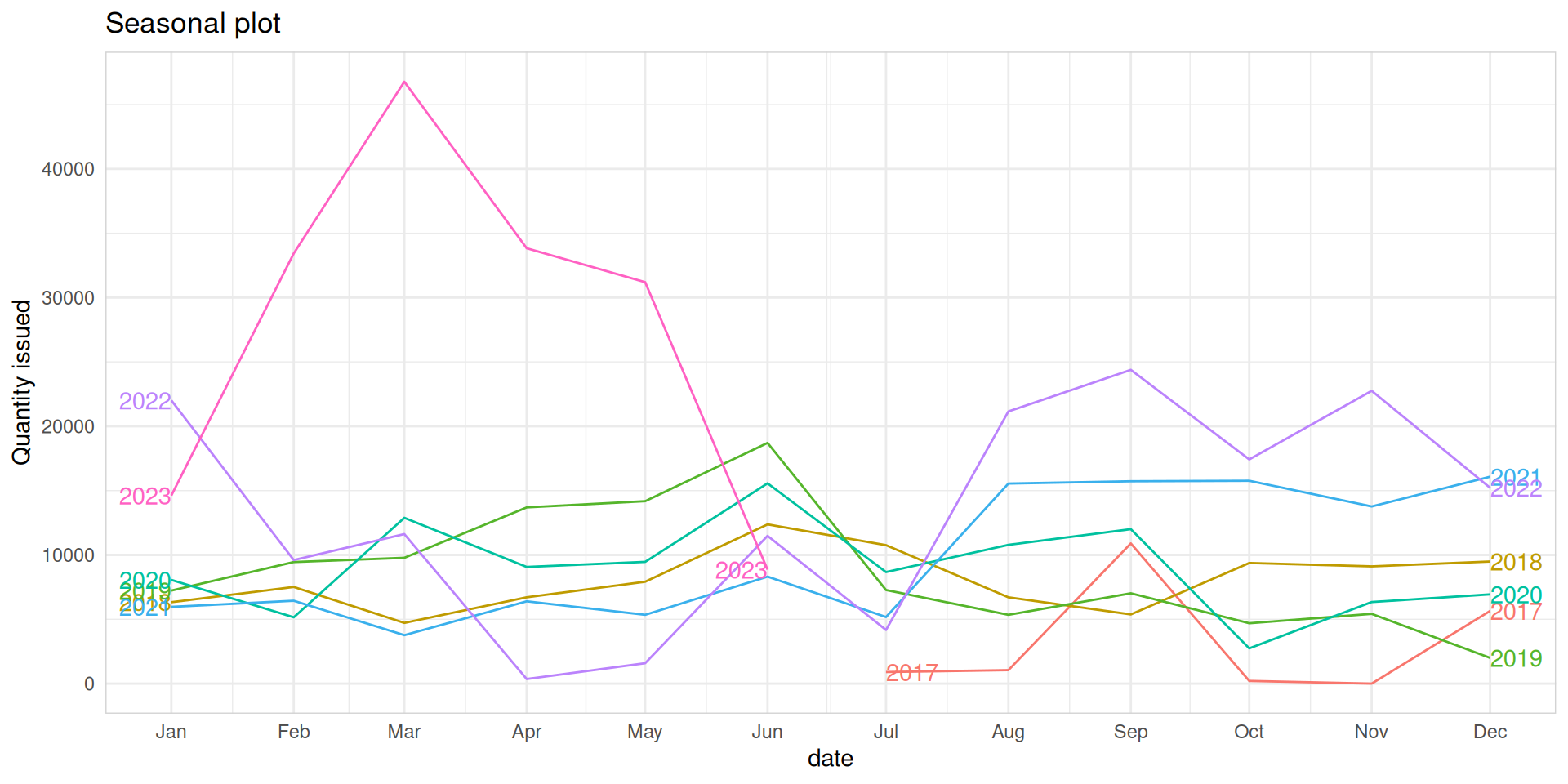
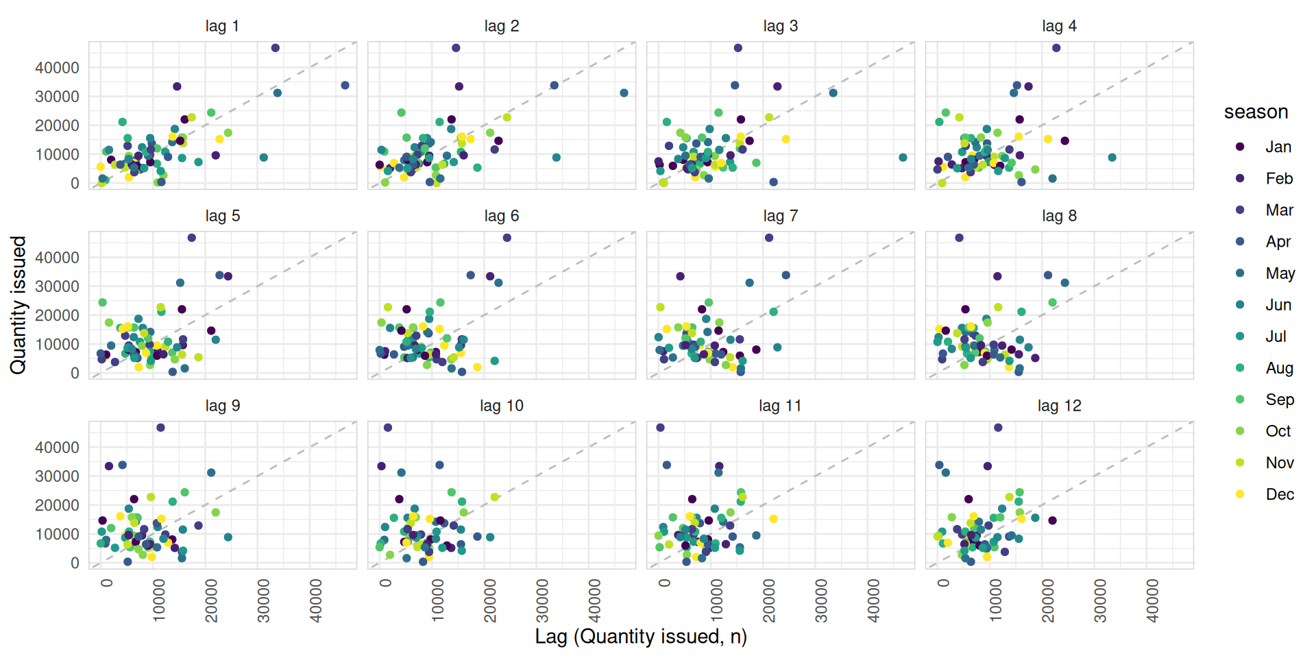
Seasonal plots
Data plotted against the individual seasons in which the data were observed (In this case a “season” is a month).
Enables the underlying seasonal pattern to be seen more clearly, and also allows any substantial departures from the seasonal pattern to be easily identified.
You can create seasonal plots using gg_season() function.
Combines Autoregressive (AR) and Moving Average (MA) components with differencing.
AR: autoregressive (lagged observations as inputs)
I: integrated (differencing to make series stationary)
MA: moving average (lagged errors as inputs)
The ARIMA model is given by:
\((1 - \phi_1 B - \dots - \phi_p B^p)(1 - B)^d y_t = c + (1 + \theta_1 B + \dots + \theta_q B^q) \epsilon_t\)
Where: \(B\): Backshift operator, \(\phi\): AR coefficients, \(\theta\): MA coefficients, \(d\): Differencing order, \(p\): AR order, \(q\): MA order and \(\epsilon_t\): White noise
ARIMA
Assumptions
Series is stationary
Linear relationship between past values and errors
White noise errors
No missing values in series
Strengths & Weaknesses
✓ Flexible for various time series patterns ✓ Perform well for short term horizons ✗ Requires stationarity for optimal performance ✗ The parameters are often not easily interpretable in terms of trend or seasonality
ARIMA
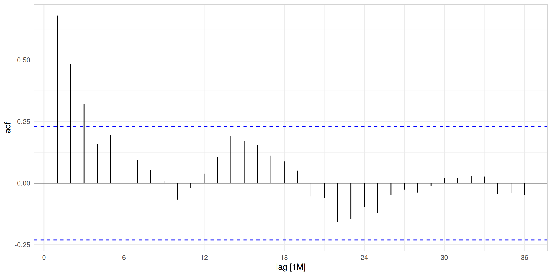
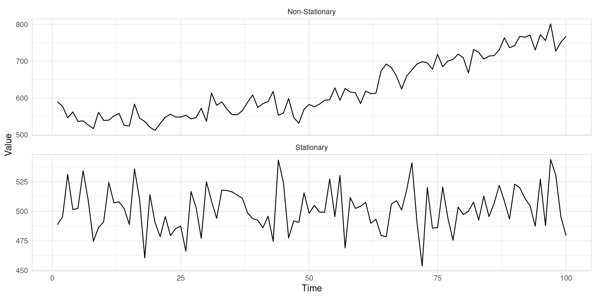
A stationary series is:
roughly horizontal
constant variance
no patterns predictable in the long-term
Seasonal ARIMA models
ARIMA
\(~\underbrace{(p, d, q)}\)
\(\underbrace{(P, D, Q)_{m}}\)
\({\uparrow}\)
\({\uparrow}\)
Non-seasonal part
Seasonal part of
of the model
of the model
\(m\): number of observations per year.
\(d\): first differences, \(D\): seasonal differences
\(p\): AR lags, \(q\): MA lags
\(P\): seasonal AR lags, \(Q\): seasonal MA lags
Seasonal and non-seasonal terms combine multiplicatively.
ARIMA automatic modelling
Plot the data. Identify any unusual observations.
If necessary, transform the data (e.g., Box-Cox transformation) to stabilize the variance.
Use ARIMA() to automatically select a model.
Check the residuals from your chosen model and if they do not look like white noise, try a modified model.
Once the residuals look like white noise, calculate forecasts.
✓ They can be adapted to various data characteristics with different error, trend, and seasonal formulations ✓ Often very effective when the underlying components are stable ✗ Parameter estimates (including smoothing parameters and initial states) can affect the forecasts ✗ May struggle to capture sudden shifts or non-standard patterns if the smoothing parameters are constant
ETS automatic modelling
Apply each model that is appropriate to the data.
Optimize parameters and initial values using MLE (or some other criterion).
The report() function gives a formatted model-specific display.
The tidy() function is used to extract the coefficients from the models.
We can extract information about some specific model using the filter() and select()functions.
Producing forecasts
The forecast() function is used to produce forecasts from estimated models.
h can be specified with:
a number (the number of future observations)
natural language (the length of time to predict)
provide a dataset of future time periods
Producing forecasts
fit_all_fc <- fit_all |>forecast(h ='year')#h = "year" is equivalent to setting h = 12.fit_all_fc
# A fable: 60 x 6 [1M]
# Key:     hub_id, product_id, .model [5]
   hub_id product_id .model     date
   <chr>  <chr>      <chr>     <mth>
 1 hub_1  product_5  naive  2023 Jul
 2 hub_1  product_5  naive  2023 Aug
 3 hub_1  product_5  naive  2023 Sep
 4 hub_1  product_5  naive  2023 Oct
 5 hub_1  product_5  naive  2023 Nov
 6 hub_1  product_5  naive  2023 Dec
 7 hub_1  product_5  naive  2024 Jan
 8 hub_1  product_5  naive  2024 Feb
 9 hub_1  product_5  naive  2024 Mar
10 hub_1  product_5  naive  2024 Apr
# ℹ 50 more rows
# ℹ 2 more variables: quantity_issued <dist>, .mean <dbl>
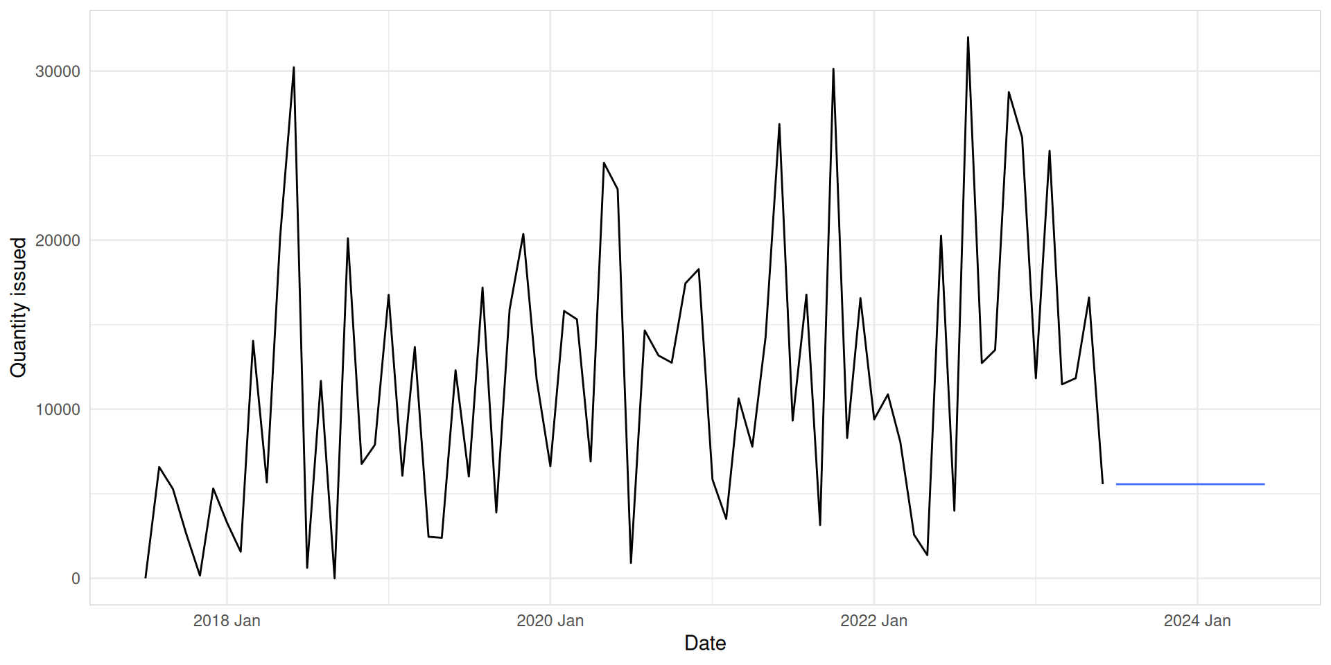
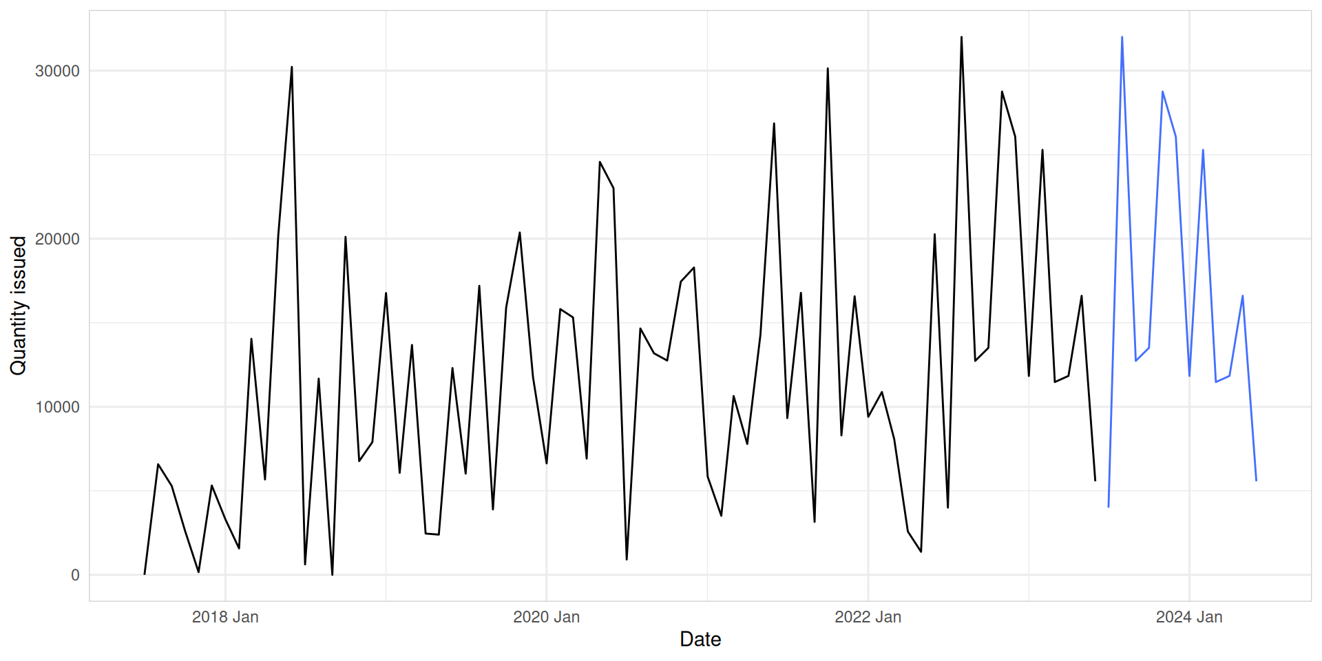
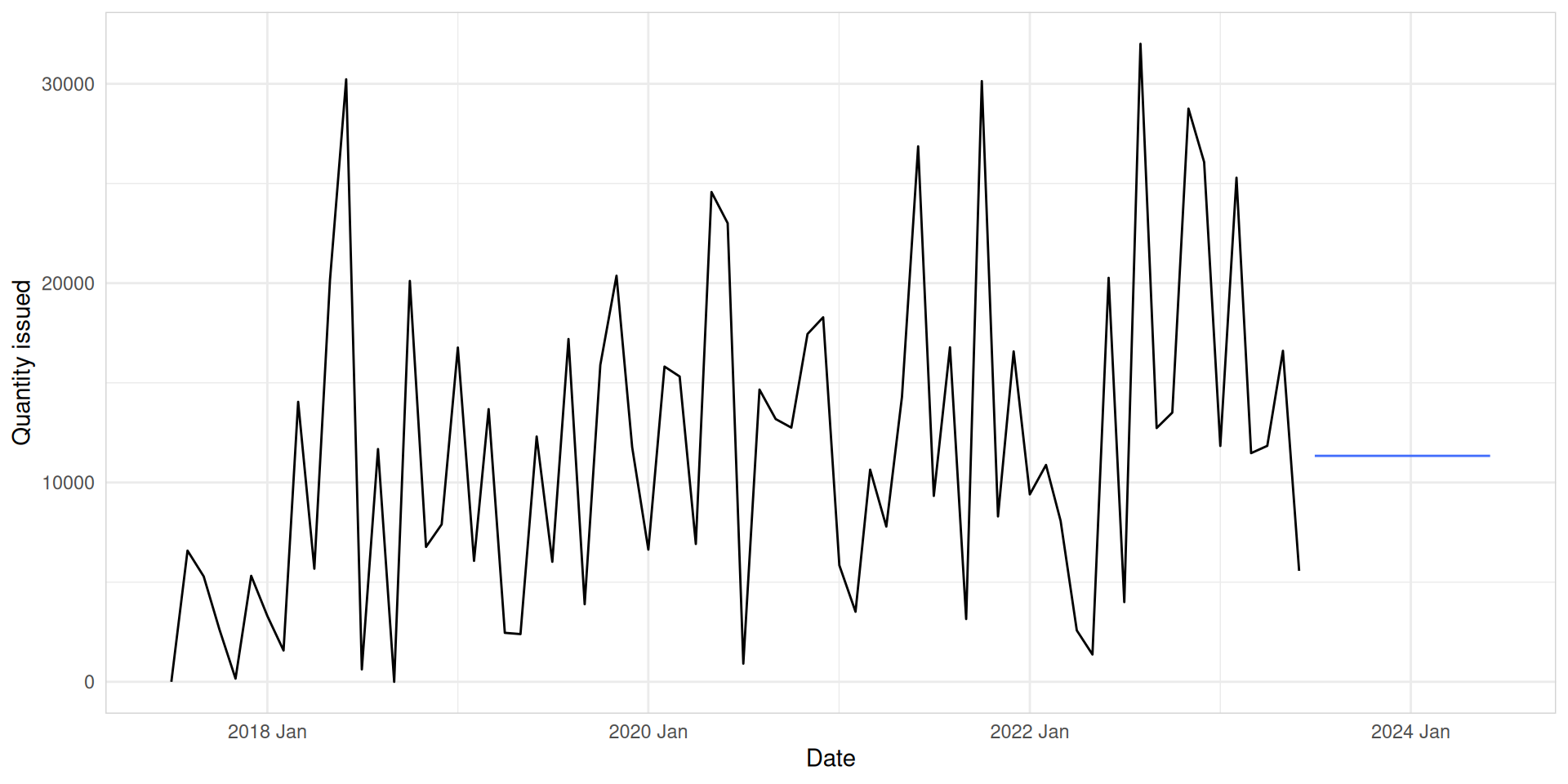
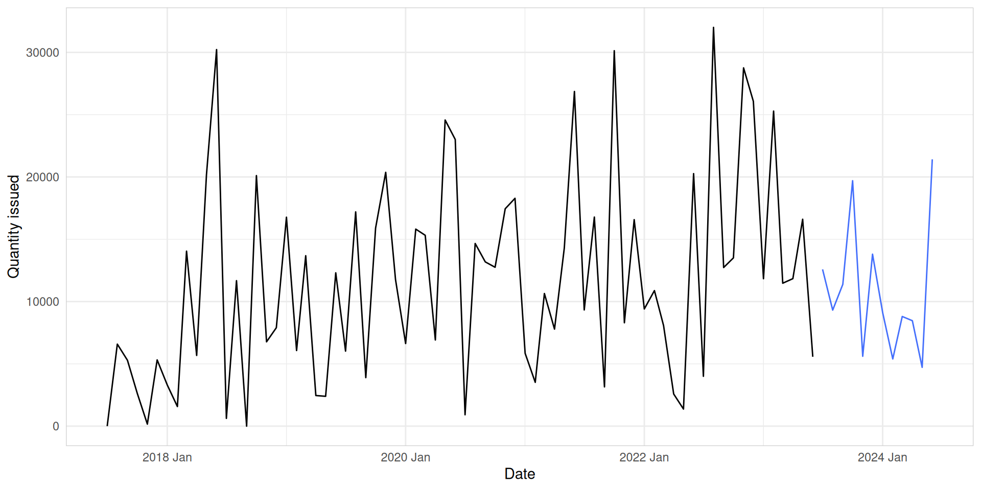
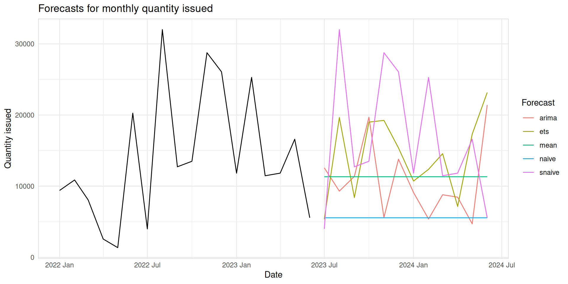
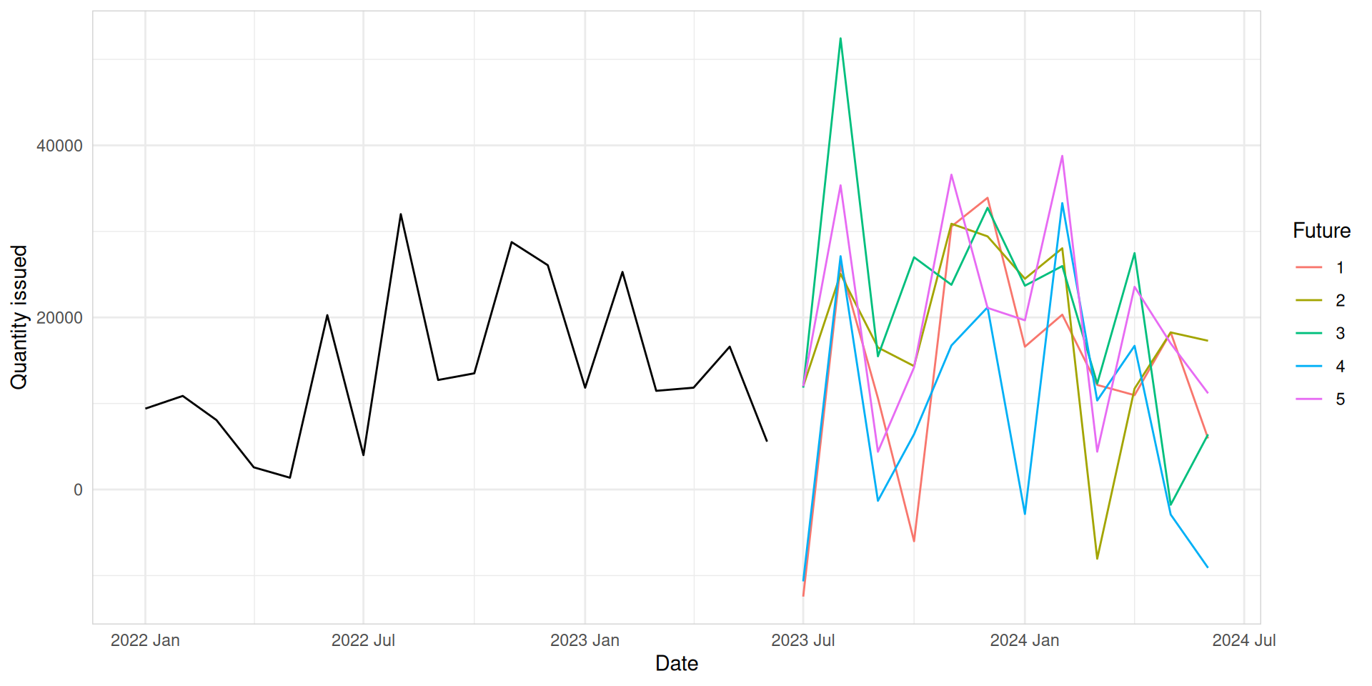
Visualising forecasts
fit_all_fc |>autoplot(level =NULL) +autolayer(med_tsb_filter |>filter_index("2022 JAn"~ .) |>filter(hub_id =='hub_1'& product_id =='product_5'), color ='black') +labs(title ="Forecasts for monthly quantity issued", y ="Quantity issued", x ="Date") +theme_minimal() +theme(panel.border =element_rect(color ="lightgrey", fill =NA)) +guides(colour=guide_legend(title="Forecast"))
Now it is your turn.
What is wrong with point forecasts?
A point forecast is a single-value prediction representing the most likely future outcome, based on current data and models.
The disadvantage of point forecast;
✗ It ignores additional information in future. ✗ It does not explain uncertainties around future. ✗ It can not deal with assymmetric.
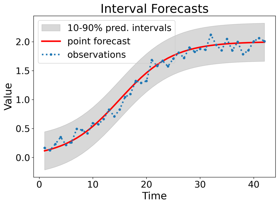
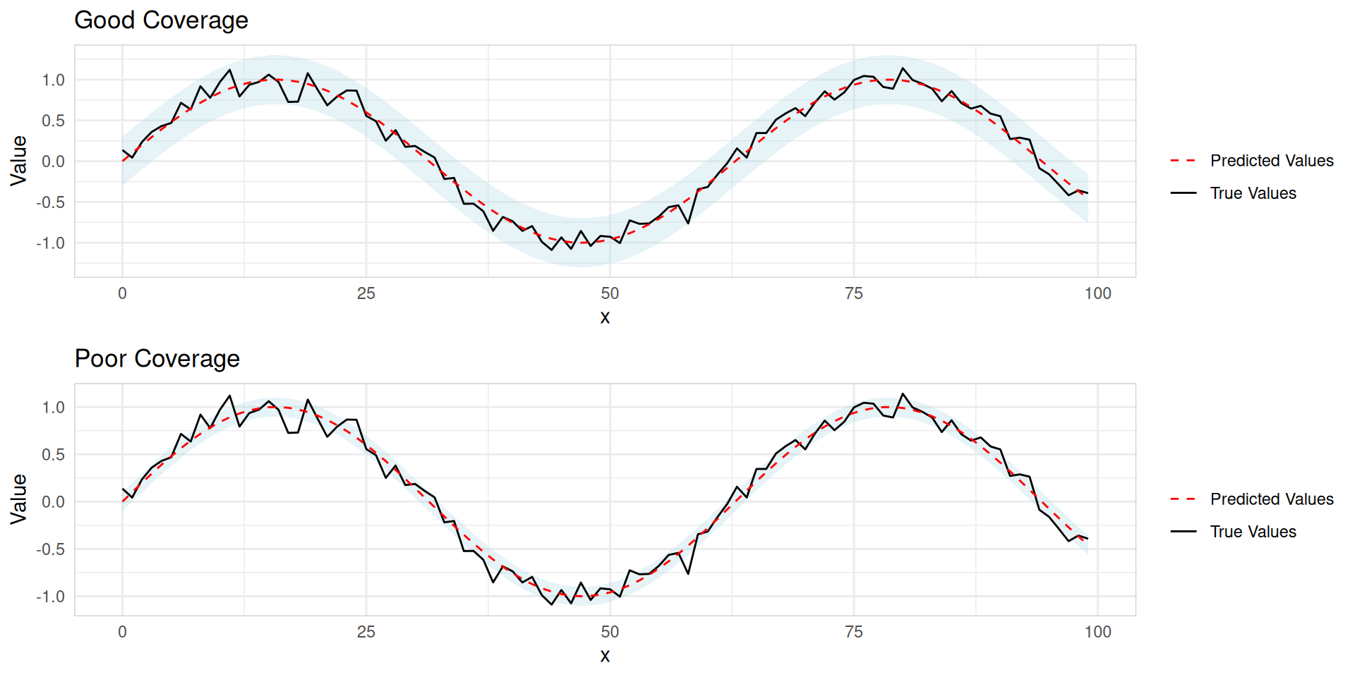
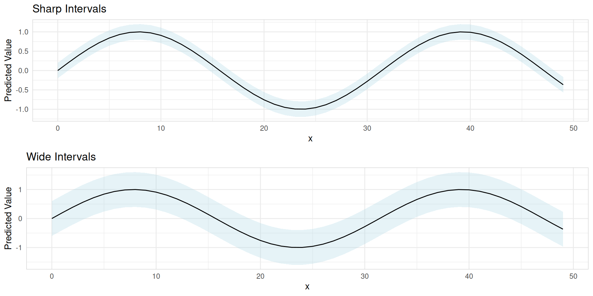
Types of probabilistic forecasts
Interval forecasts: A prediction interval is an interval within which power generation may lie, with a certain probability.
Types of probabilistic forecasts
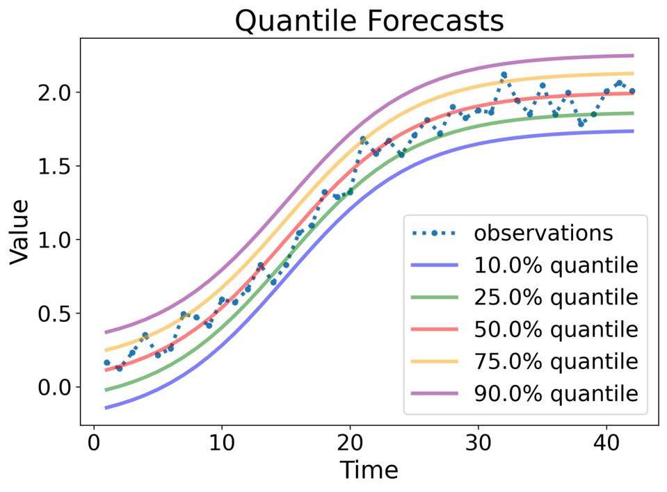
Quantile forecasts: A quantile forecast provides a value that the future observation is expected to be below with a specified probability.
Types of probabilistic forecasts
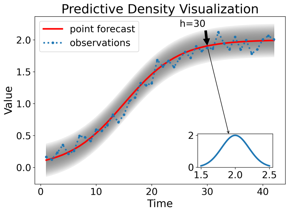
Distribution forecasts: A comprehensive probabilistic forecast capturing the full range of potential outcomes across all time horizons.
Types of probabilistic forecasts
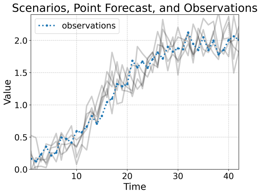
Scenario forecasts: A spectrum of potential futures derived from probabilistic modeling to inform decision- making under uncertainty.
Forecast distributions from bootstrapping
When a normal distribution for the residuals is an unreasonable assumption, one alternative is to use bootstrapping, which only assumes that the residuals are uncorrelated with constant variance.
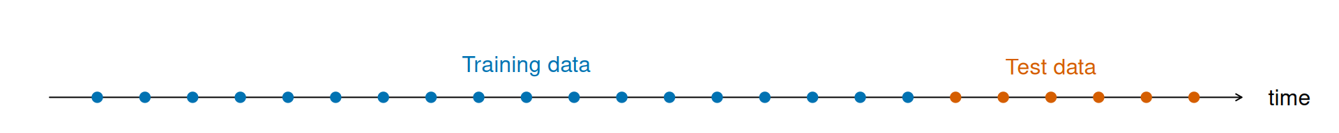
We pretend we don’t know some part of data (new data)
It must not be used for any aspect of model training
Forecast accuracy is computed only based on the test set
Training and test sets
Evaluating point forecast accuracy
In order to evaluate the performance of a forecasting model, we compute its forecast accuracy.
Forecast accuracy is compared by measuring errors based on the test set.
Ideally it should allow comparing benefits from improved accuracy with the cost of obtaining the improvement.
Evaluating point forecast accuracy
Forecast Error
\(e_{T+h} = y_{T+h} - \hat{y}_{T+h\mid T}\)
where
- \(y_{T+h}\) is the \((T+h)^\text{th}\) observation \((h=1,\dots,H)\), and
- \(\hat{y}_{T+h\mid T}\) is the forecast based on data up to time \(T\).
Scale independent; use if \(y_t \gg 0\) and \(y\) has a natural zero
RMSE (Root Mean Squared Error)
\(\text{RMSE} = \sqrt{\text{mean}(e_{T+h}^2)}\)
Scale dependent
Evaluating point forecast accuracy
Measure
Formula
Notes
MASE (Mean Absolute Scaled Error)
\(\text{MASE} = \text{mean}(|e_{T+h}|/Q)\)
Non-seasonal:\(Q = \frac{1}{T-1}\sum_{t=2}^T |y_t-y_{t-1}|\) Seasonal:\(Q = \frac{1}{T-m}\sum_{t=m+1}^T |y_t-y_{t-m}|\), where \(m\) is the seasonal frequency
Non-seasonal:\(Q = \frac{1}{T-1}\sum_{t=2}^T (y_t-y_{t-1})^2\) Seasonal:\(Q = \frac{1}{T-m}\sum_{t=m+1}^T (y_t-y_{t-m})^2\), where \(m\) is the seasonal frequency
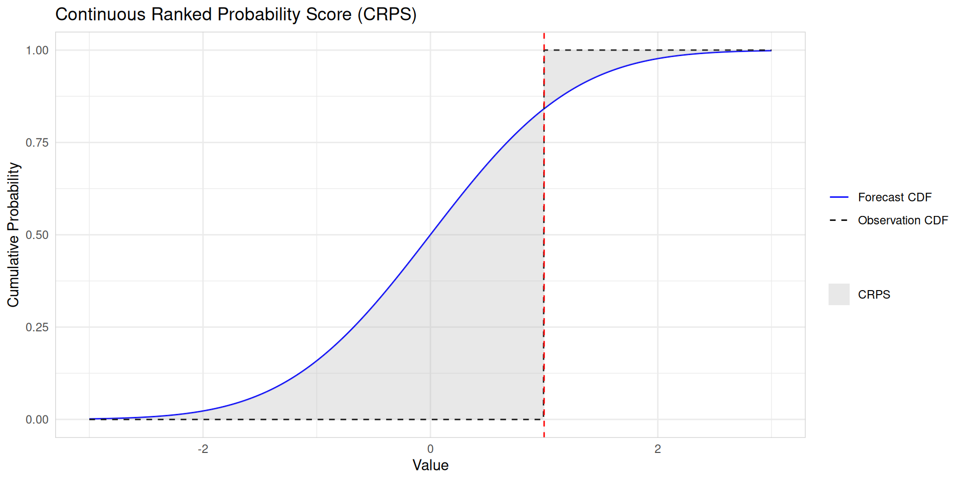
# A tibble: 5 × 5
  .model hub_id product_id .type  CRPS
  <chr>  <chr>  <chr>      <chr> <dbl>
1 arima  hub_1  product_5  Test  6311.
2 ets    hub_1  product_5  Test  6648.
3 mean   hub_1  product_5  Test  7081.
4 naive  hub_1  product_5  Test  8034.
5 snaive hub_1  product_5  Test  7823.
Now it is your turn.
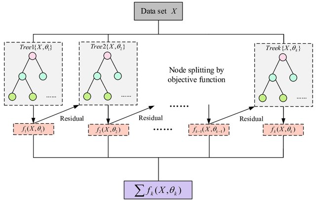
Advance forecasting models
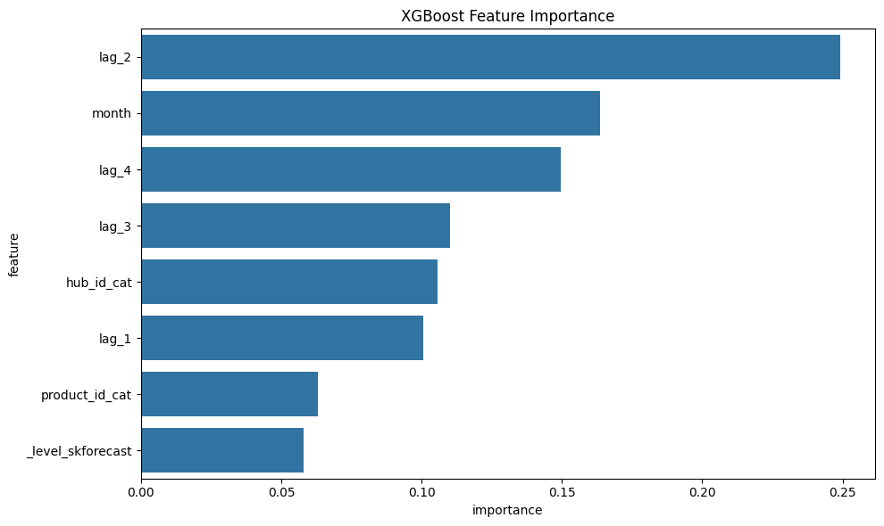
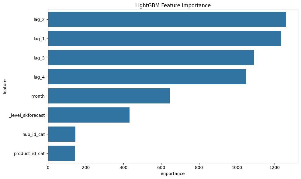
Feature engineering
In this training, we only do a basic feature engineering.
# Load datafrom google.colab import filesuploaded = files.upload()df = pd.read_csv('med_tsb_filter.csv')# Make the yearmonth as date formatdf['date'] = pd.to_datetime(df['date']) + pd.offsets.MonthEnd(0)# Feature Engineeringdf['month'] = df['date'].dt.month # create month feature# categorical encodingenc = OrdinalEncoder()df[['hub_id_cat', 'product_id_cat']] = enc.fit_transform(df[['hub_id', 'product_id']])# Create unique identifier for seriesdf['unique_id'] = df['hub_id'] +'_'+ df['product_id']
Feature engineering
# Create series and exogenous dataseries = df[['date', 'unique_id', 'quantity_issued']]exog = df[['date', 'unique_id', 'month', 'hub_id_cat', 'product_id_cat']]# Transform series and exog to dictionariesseries_dict = series_long_to_dict( data = series, series_id ='unique_id', index ='date', values ='quantity_issued', freq ='M')exog_dict = exog_long_to_dict( data = exog, series_id ='unique_id', index ='date', freq ='M')
Feature engineering
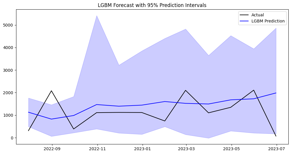
# Partition data in train and testend_train ='2022-06-30'start_test = pd.to_datetime(end_train) + pd.DateOffset(months=1) # Add 1 monthseries_dict_train = {k: v.loc[:end_train] for k, v in series_dict.items()}exog_dict_train = {k: v.loc[:end_train] for k, v in exog_dict.items()}series_dict_test = {k: v.loc[start_test:] for k, v in series_dict.items()}exog_dict_test = {k: v.loc[start_test:] for k, v in exog_dict.items()}
# Since we already have done the feature engineering, we dont need to do it again# Create unique identifier and rename columns for TimeGPTdf_timegpt = df.rename(columns={'date': 'ds', 'quantity_issued': 'y'}).drop(columns=['hub_id', 'product_id'])# Split data into train-testend_train ='2022-06-30'train_df = df_timegpt[df_timegpt['ds'] <= end_train]test_df = df_timegpt[df_timegpt['ds'] > end_train]
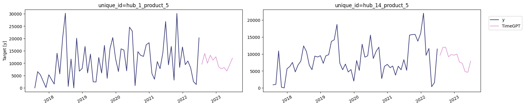
TimeGPT
# TimeGPT Base Modeltimegpt_fcst = nixtla_client.forecast( df=train_df, h=len(test_df['ds'].unique()), freq='M', level=[90, 95] # 90% and 95% prediction intervals)nixtla_client.plot(train_df, timegpt_fcst, time_col='ds', target_col='y')
\(\text{mCPR}\): Modern Contraceptive Prevalence Rate (%)
\(\text{WomenPopulation}\): Women aged 15-49
\(\text{MethodMix}\): Contraceptive method distribution
\(\text{CYP}\): Couple-Years of Protection factor
\(\text{BrandMix}\): Brand preference distribution
\(\text{SourceShare}\): Provider type distribution
Demographic forecasting method (FPSC Context)
Assumptions
Stable demographic patterns during forecast period
Consistent reporting of family planning indicators
Accurate CYP values for different methods
Historical brand/source mixes remain valid
Linear relationship between population and needs
Proper spatial distribution via site coordinates
Valid monthly weight distribution
Demographic forecasting method (FPSC Context)
Strengths & Weaknesses
✓ Directly ties to population dynamics ✓ Incorporates multiple programmatic factors ✓ Enables spatial allocation to health sites ✓ Aligns with public health planning frameworks ✗ Sensitive to input data quality ✗ Static assumptions about behavior patterns ✗ Limited responsiveness to sudden changes ✗ Provides national level need
Demographic forecasting method (FPSC Context)
Female condom needs (age 20-15) for 2020 (example)
Parameter
Value
Unit
Sources
A. Women population 20 – 25
345,000
# of people
WorldPop
B. Percentage of women who will use a contraceptive product (mCPR)