Cardiff University Logo Data Lab Logo HISP UIO Logo DHIS2 Logo WGSSS Logo UKRI Logo

Live Demo

Leveraging Chap and the DHIS2 Platform for Stock Forecasting

Data Lab for Social Good Research Group in collaboration with HISP Centre, University of Oslo

2026/01/27


Outline

Background

The fundamental question

What we are going to do

What did we find

Live demo

BACKGROUND

The Problem: A tale of two data streams


Health supply chains are struggling with forecasting at sub-national/ facility level.

  • Operational realities: Incomplete records, irregular orders, frequent manual adjustments.

  • This masks true demand and leads to a cycle of persistent, critical stockouts.


But… we have a success story.


Platforms like DHIS2 and CHAP have robust, high-performing models for forecasting disease cases (morbidity).

The fundemental question


✅ We’re good at forecasting cases (e.g., malaria).


❌ We’re struggling with forecasting consumption (e.g., antimalarials) at sub-national level.


Can the same CHAP morbidity models and pipelines be ported to health commodity demand and inventory decisions?


Portability lens

  • Same platform (DHIS2/CHAP)
  • Same model pipelines
  • New target (consumption)

The challenge: Why isn’t this easy?


Case data and consumption data are different.


Different Data Structures

Consumption data is “messier”.

  • Missing entries (e.g., “0” = no consumption, or “0” = data not entered?)
  • Intermittency (infrequent demand).
  • Inconsistent recording.

Different Metadata

Consumption is affected by logistics.

  • Lead times.
  • Procurement cycles.
  • Existing stock levels and stockouts.

OUR APPROACH

What we are going to do


Apply the same CHAP morbidity models (no extra tuning) to product demand (malaria commodities, vaccines).


Link forecasts to operations: evaluate both forecast accuracy and inventory impact.


Build a portability matrix: when can we transfer a model?


Design an implementation workflow for DHIS2/CHAP.


Provide R scripts, CHAP YAML configs and sample datasets for full reproducibility.

Why forecasting is not “one AI model”


In practice, forecasting relies on many different types of models, each designed for different data patterns and decisions.

This is where CHAP within DHIS2 differs from AI agents: CHAP is model-agnostic. It lets users run, compare, and select models, rather than delegating all decisions to a single AI agent.

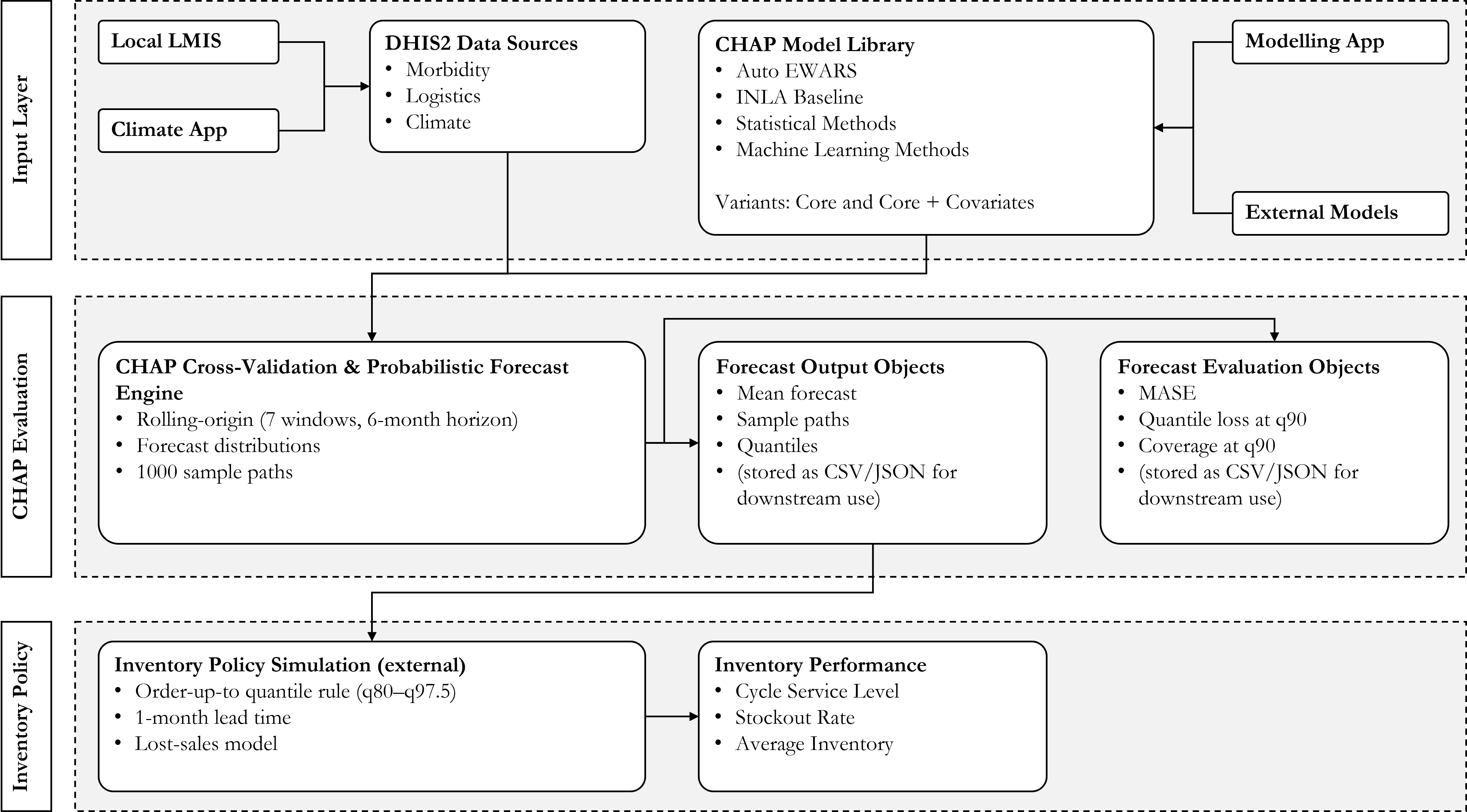
Our experimental workflow


Data sources


Data source Domain Geography / Sites Coverage period Granularity
DHIS2 Dengue cases Brazil (23 locations) 2001 Jan – 2017 Dec Monthly, subnational
Laos (7 locations) 2000 Jul – 2013 Jun Monthly, subnational
Paraguay (16 locations) 2012 Mar – 2017 Dec Monthly, subnational
Vietnam (19 locations) 2000 Jul – 2017 Jun Monthly, subnational
DHIS2 Malaria incidence Rwanda (30 locations) 2015 Jan – 2024 Dec Monthly, subnational
DHIS2 / LMIS Malaria commodities Laos (11 products, 18 facilities) 2019 Feb – 2021 Jun Monthly, subnational
DHIS2 / LMIS Vaccine consumption Laos (21 products, 10 facilities) 2021 Feb – 2024 Jan Monthly, subnational
DHIS2 Climate App Climate covariates All study settings Study-specific Monthly, subnational

Overview of the candidate models

Method Covariates
Auto EWARS Population, rainfall, teamperature
INLA Baseline None
Naïve None
sNaive None
Mean None
ETS None
ARIMA None
ARIMA Climate Rainfall, temperature
ARIMA Madagaskar Rainfall (Lag 3), temperature (Lag 3)
Linear Regression Trend, seasonality
Linear Regression Climate Trend, seasonality, rainfall, teamperature
LightGBM Percentage of zero values, lags of target variable (lag 6 - 12), rainfall, temperature, month, healthcare facility code, product code
XGBoost Percentage of zero values, lags of target variable (lag 6 - 12), rainfall, temperature, month, healthcare facility code, product code
Random Forest Percentage of zero values, lags of target variable (lag 6 - 12), rainfall, temperature, month, healthcare facility code, product code

FINDINGS

Data exploration

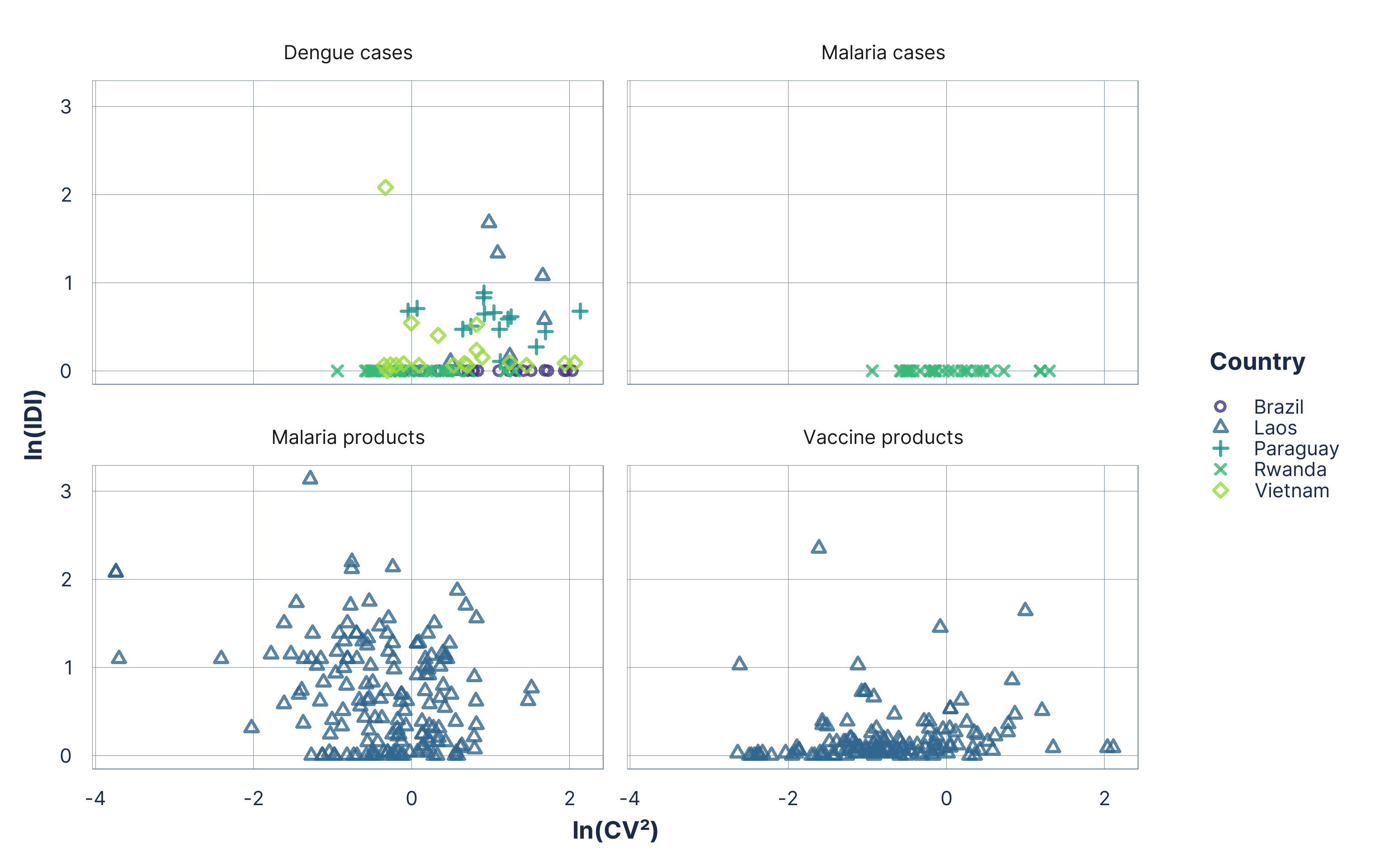
Figure 1: Classification of all morbidity and consumption series using the ln(CV²) and ln(IDI) map. Each point represents a monthly series plotted on the logarithmic CV²–IDI scale.

Average forecast method rankings

Figure 2: Average point forecast (MASE) ranks. Methods on the y-axis are ordered from best (top) to worst (bottom) based on their overall average rank across all domains. Lower ranks indicate better performance.

Average forecast method rankings

Figure 3: Average probabilistic forecast (quantile loss) ranks. Methods on the y-axis are ordered from best (top) to worst (bottom) based on their overall average rank across all domains. Lower ranks indicate better performance.

Overall inventory performance - Malaria products

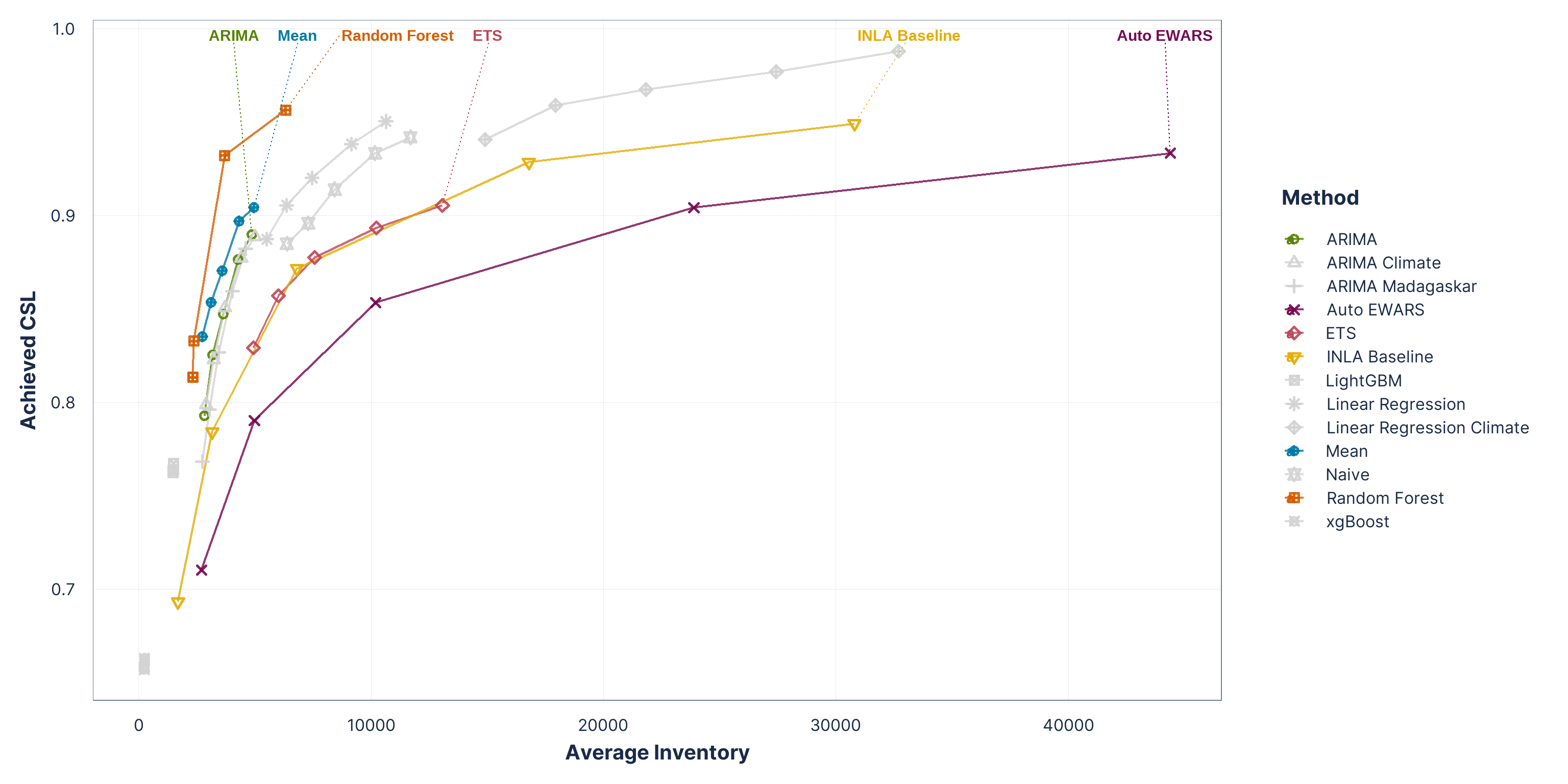
Figure 4: Inventory performance across malaria-product simulations using quantile-based order-up-to policies (q80–q97.5).

Overall inventory performance - Vaccine

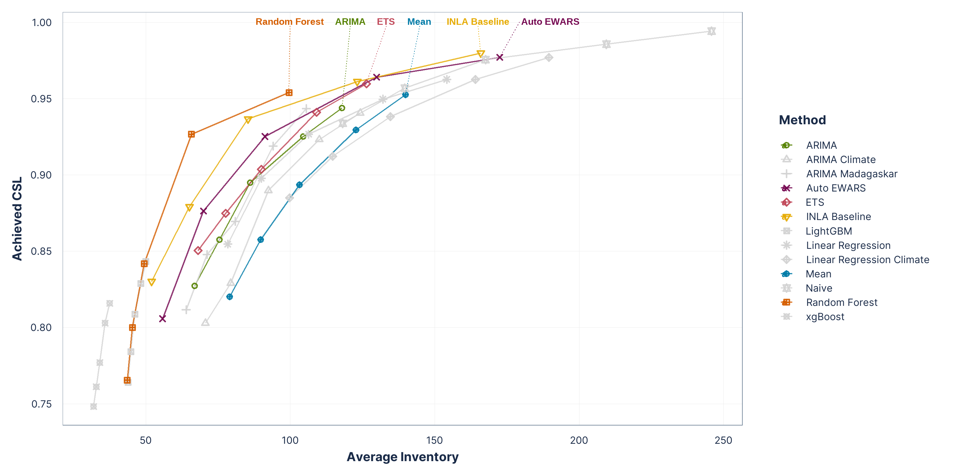
Figure 5: Inventory performance across vaccine-product simulations using quantile-based order-up-to policies (q80–q97.5).

Execution scalability of all forecasting methods

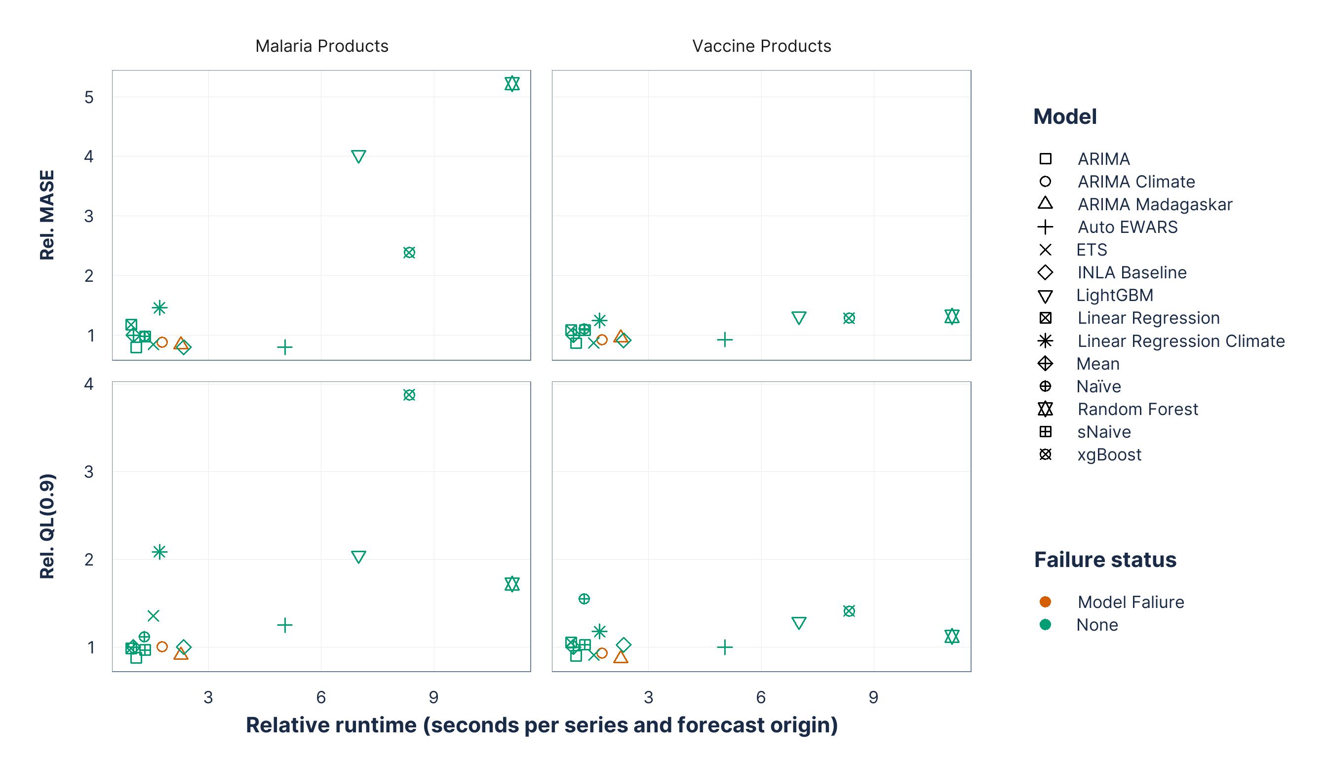
Figure 6: Model portability metrics for all candidate forecasting methods, relative to the Mean method. Relative MASE and QL(0.9) are reported separately for malaria and vaccine products; values below 1 indicate improvement over the Mean method.

What does this mean for supply chain forecasting?


Can the same DHIS2 / CHAP platform be used for supply chain forecasting?

Yes, the platform is generic and extensible beyond disease surveillance.


Can one model work well for all supply chain problems?

Not really, demand patterns, data quality, and decision contexts differ. However, a small set of models tend to perform consistently well across settings.


How does CHAP handle this heterogeneity?

CHAP gives full autonomy to plug in, test, and select models based on the use case, rather than enforcing a single “best” model.


Do we need system-level adaptations for supply chains?

Yes, modest but important tweaks are needed (data structures, evaluation metrics, and decision-oriented outputs).

LIVE DEMO

Resources


GitHub repo with all R codes and YML configurations


Documentation for Model Developers


Running models through Chap


Configure DHIS2 Modeling App and Chap Core


Pay Attention

This demo shows how existing CHAP pipelines can run external forecasting and inventory models using external data, without modifying core workflows; therefore, some variables are renamed purely for schema compatibility (e.g., dispensed → disease_cases), with no change to data meaning or modelling logic.

Minimalistic model example using R

# List packages
library(tidyverse)
library(fable)
library(tsibble)

# train models - # auto ets model 

train_chap <- function(csv_fn, model_fn) {
  df <- read_csv(csv_fn) |> 
    mutate(target = if_else(is.na(target), 0, target),
           time_period = yearmonth(time_period))
  
  df <- df |> distinct() |> 
    as_tsibble(index = time_period, key = location) |> 
    fill_gaps(target=0L, .full = TRUE)
  
  model <- df |> 
    model(ets = ETS(target))
  
  saveRDS(model, file=model_fn)
  
  print('train done')
  
}

args <- commandArgs(trailingOnly = TRUE)

if (length(args) == 2) {
  csv_fn <- args[1]
  model_fn <- args[2]
  
  train_chap(csv_fn, model_fn)
}# else {
#  stop("Usage: Rscript train.R <csv_fn> <model_fn>")
#}
# Load required libraries
library(tidyverse)
library(fable)
library(tsibble)

# Define the predict function
predict_chap <- function(model_fn, historic_data_fn, future_climatedata_fn, predictions_fn) {
  
  # Load the pre-trained model structure
  model <- readRDS(model_fn)
  
  print('read model')
  
  # Load the complete historical data
  historic_df <- read_csv(historic_data_fn) |>
    mutate(target = if_else(is.na(target), 0, target),
           time_period = yearmonth(time_period)) |>
    as_tsibble(index = time_period, key = location) |> 
    fill_gaps(target=0L, .full = TRUE) 
  
  # Load the future data (covariates only)
  future_df <- read_csv(future_climatedata_fn) |>
    mutate(time_period = yearmonth(time_period)) |>
    as_tsibble(index = time_period, key = location)
  
  print('load_data')
  
  # Refit the model with all historic data and forecast
  
  model <- model |>
    refit(historic_df)
  
  y_pred <- model |>
    generate(new_data = future_df, bootstrap = FALSE, times = 1000) |> 
    mutate(.rep = as.integer(.rep)) |> 
    arrange(.rep) |> 
    pivot_wider(names_from = .rep, values_from = .sim, names_prefix = "sample_")
  
  print(y_pred)
  
  # saveRDS(model, file = model_fn)
  
  df_out <- future_df |>
    left_join(y_pred |>
                select(-.model) |> 
                mutate(across(starts_with("sample_"), ~ if_else(. < 0, 0, .))) |>
                rename_with(~ paste0("sample_", as.integer(str_extract(., "\\d+")) - 1), starts_with("sample_")),
              by = c('location', 'time_period')
    ) |>
    as_tibble() |>
    mutate(time_period = format(as.Date(time_period), "%Y-%m")) |> 
    select(time_period, location, starts_with("sample_"))
  
  
  print('made predictions')
  
  df_out |> print()
  
  
  write.csv(df_out, predictions_fn, row.names = FALSE)
  
  fname <- paste0("df_out_", format(Sys.time(), "%Y%m%d_%H%M%S"), predictions_fn)
  write_csv(y_pred, fname)
  
}

# --- Command Line Argument Handling (No change here) ---

args <- commandArgs(trailingOnly = TRUE)

if (length(args) == 4) {
  model_fn <- args[1]
  historic_data_fn <- args[2]
  future_climatedata_fn <- args[3]
  predictions_fn <- args[4]
  
  predict_chap(model_fn, historic_data_fn, future_climatedata_fn, predictions_fn)
}

# Inventory sim

source('quantile_based_inventory_sim.R')
source("ets-r/train.R")
source("ets-r/predict.R")

train_chap("ets-r/training_data.csv", 
           "ets-r/output/model.bin")

predict_chap("ets-r/output/model.bin", 
             "ets-r/historic_data.csv", 
             "ets-r/future_data.csv", 
             "ets-r/predictions.csv")
name: ets-r

target: disease_cases

adapters: {'target': 'disease_cases'}

docker_env:
  image: ets-r:latest

entry_points:
  train:
    parameters:
      train_data: path
      model: path
    command: "Rscript train.R {train_data} {model}"
  predict:
    parameters:
      historic_data: path
      future_data: path
      model: str
      out_file: path
    command: "Rscript predict.R {model} {historic_data} {future_data} {out_file}"
FROM ghcr.io/dhis2-chap/docker_r_inla:master

RUN apt-get update
RUN apt-get install -y libharfbuzz-dev libfribidi-dev
RUN R -e 'r = getOption("repos"); r["CRAN"] = "http://cran.us.r-project.org"; options(repos = r); install.packages(c("tidyverse", "fable", "tsibble", "fabletools", "fpp3", "doParallel"), repos=c(getOption("repos"), dep=TRUE))'

Inventory policy: Order-upto-level with lost sales

# Inventory simulation

library(tidyverse)
library(tsibble)
library(doParallel)

set.seed(100)

# Read data ---------------------------------------------------------------

actual_df <- read.csv('data/laos/laos_epi_cleaned.csv') |> 
  rename(date = time_period,
         dispensed = disease_cases) |> 
  select(date, location, dispensed) |> 
  as_tibble()

pred_all <- read.csv('predictions.csv')

pred_master_df <- pred_all |> 
  rename(date = time_period) |> 
  mutate(across(starts_with("sample"), ~ pmax(., 0))) |> 
  rowwise() |> 
  mutate(
    mean = mean(c_across(starts_with("sample")), na.rm = TRUE) * 3,
    q80  = quantile(c_across(starts_with("sample")), probs = 0.80, na.rm = TRUE, names = FALSE),
    q85  = quantile(c_across(starts_with("sample")), probs = 0.85, na.rm = TRUE, names = FALSE),
    q90  = quantile(c_across(starts_with("sample")), probs = 0.90, na.rm = TRUE, names = FALSE),
    q95  = quantile(c_across(starts_with("sample")), probs = 0.95, na.rm = TRUE, names = FALSE),
    q975 = quantile(c_across(starts_with("sample")), probs = 0.975, na.rm = TRUE, names = FALSE)
  )  |> 
  ungroup() |> 
  select(date, location, mean, q80, q85, q90, q95, q975)

master_df <- pred_master_df |> 
  left_join(actual_df, by = c('date', 'location')) |> 
  mutate(date = as.Date(paste0(date, "-01")))
# Inventory function ------------------------------------------------------

master_long <- master_df |> 
  # filter(location == '0701larmany-0701 Xamnua-BCG diluent' & model == 'ETS') |> 
  pivot_longer(cols = c('mean', 'q80', 'q85', 'q90', 'q95', 'q975'), names_to = 'target_csl', values_to = 'quantity') |> 
  mutate(id = paste0(location, ':', target_csl))

id_list <- master_long |> 
  pull(id) |> 
  unique() 

# Register outer parallel backend with multiple cores

n_cores <- detectCores(logical = FALSE) - 1   # 16 physical cores – 1 = 15
cl_outer <- makeCluster(n_cores)
registerDoParallel(cl_outer)

# parallel loop

system.time(inventory_sim_full <- foreach(i = id_list,
                                          .combine = 'rbind',
                                          .packages=c("doParallel", "foreach", "tidyverse", "tsibble", "fable")) %dopar% {
                                            
                                            # i <- id_list[1]
                                            
                                            df <- master_long |>
                                              filter(id == i) |> 
                                              group_by(location, target_csl) |> 
                                              arrange(date) |>
                                              mutate(
                                                target_stock = quantity,
                                                opening_stock = 0,
                                                received = 0,
                                                closing_stock = 0,
                                                order_qty = 0,
                                                delivery_due = NA,
                                                fixed_lead_time = 1
                                              )
                                            
                                            deliveries <- list()
                                            
                                            for (i in seq_len(nrow(df))) {
                                              today <- df$date[i]
                                              
                                              # Receive orders
                                              arrivals <- deliveries |>
                                                keep(~.x$arrival_date == today) |>
                                                map_dbl("amount") |>
                                                sum()
                                              
                                              df$opening_stock[i] <- if (i == 1) arrivals else df$closing_stock[i - 1] + arrivals
                                              actual <- df$dispensed[i]
                                              
                                              df$received[i] <- arrivals
                                              df$closing_stock[i] <- max(0, df$opening_stock[i] - actual)
                                              
                                              # Place order
                                              order_qty <- max(0, df$target_stock[i] - df$closing_stock[i])
                                              lead_time <- df$fixed_lead_time[i]
                                              delivery_date <- today %m+% months(lead_time)
                                              
                                              deliveries <- append(deliveries, list(list(arrival_date = delivery_date, amount = order_qty)))
                                              
                                              df$order_qty[i] <- order_qty
                                              df$delivery_due[i] <- delivery_date
                                            }
                                            
                                            
                                            inventory_sim <- df |>
                                              mutate(
                                                lost_sales = pmax(0, dispensed - pmin(dispensed, opening_stock)),
                                                met_demand = dispensed <= opening_stock,
                                                stockout = dispensed > opening_stock
                                              )
                                            
                                            inventory_sim
                                            
                                          })

# Stop outer cluster

stopCluster(cl_outer)


# Final data

write_csv(inventory_sim_full, 'inventory_sim.csv')


# Inventory value added ---------------------------------------------------

inv_metrics <- inventory_sim_full |> 
  group_by(location, target_csl) |> 
  slice(-1) |> 
  summarise(
    CSL = round(mean(met_demand, na.rm=TRUE), 1),
    stockout_rate = round(mean(stockout, na.rm=TRUE), 1),
    avg_inventory = round(mean(mean((opening_stock+closing_stock)/2, na.rm=TRUE), 1)),
    # avg_inventory = round(mean(if_else(order_qty >= 0.1,
    #                                     ((opening_stock+closing_stock)/2)/order_qty, NA_real_), 
    #                             na.rm=TRUE), 1),
    .groups        = "drop"
  )

fname <- paste0("df_out_", format(Sys.time(), "%Y%m%d_%H%M%S"), 'inventory.csv')
write_csv(inv_metrics, fname)

Running models through Chap (docker + WSL)


Connect with CHAP Core

cd chap-core/

source .venv/bin/activate


Create docker image

cd /mnt/d/GIT/dhis2_demo/ets-r

docker build -t ets-r:latest .

# Return to CHAP Core

cd ~

cd chap-core/


Run CHAP evaluation

chap evaluate --model-name /mnt/d/GIT/dhis2_demo/ets-r --dataset-csv /mnt/d/GIT/dhis2_demo/ets-r/data/laos/laos_epi_cleaned.csv

Any questions or thoughts? 💬