![]()
![]()


Seen the UNSEEN

This is Nilu.
She went to the pharmacy today to get contraceptive Product A.
But it wasn’t in stock.
Seen the UNSEEN

She didn’t go to the pharmacy today.
Why would she?
The last two times she went, they didn’t have the product she needed.
The system doesn’t know this.
It sees “no demand” and it continously logs Nilu’s silence as data.
Seen the UNSEEN
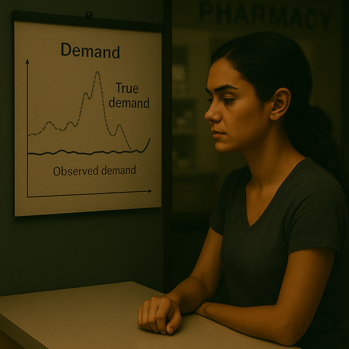
When data is censored by stockouts or service interruptions…
…forecasts fail.
Not just by being wrong, But by being blind.
This creates a broken trust and leads to
UNMET DEMAND.
Seen the UNSEEN

In reality…
There are more than
218 million women
like Nilu still have an unmet need for family planning.
Ultimately, this results in dropouts, unwanted pregnancies, and almost 7 million hospitalizations each year in developing countries.
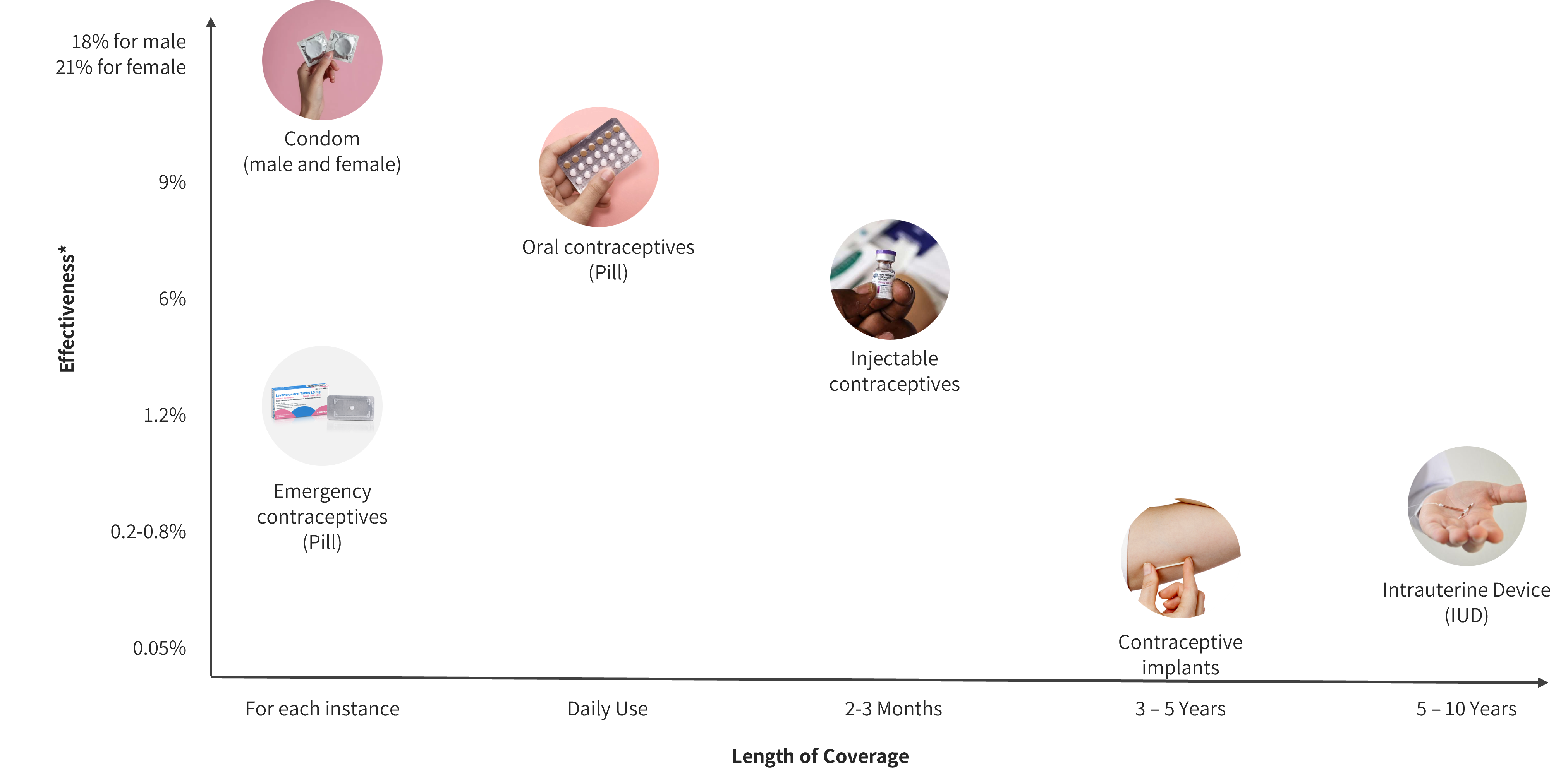
Contraceptive products aren’t easily SUBSTITUTED
Censorship scenarios
How can a demand forecasting and inventory optimization model that incorporates lost sales estimation and contextual field data enhance contraceptive supply chain performance and reduce stockouts in developing countries?
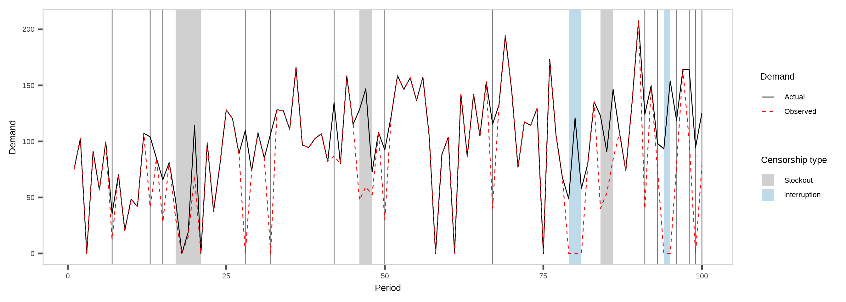
Figure 1: Censorship scenarios in family planning supply chains.
Why this is critical
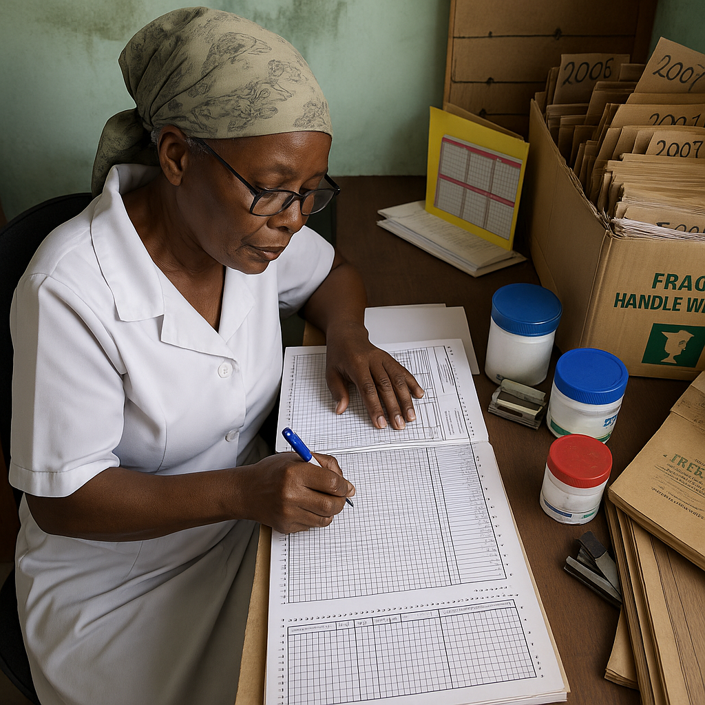
- Frequent stockouts are common in family planning supply chains, especially in developing countries, significantly impacting public health outcomes.
- During my recent field visit to Ethiopia, stockouts were repeatedly identified by demand planners as a major barrier to effective contraceptive supply management.
- Traditional forecasting methods fail under censorship.
- Prior research inadequately addresses demand estimation under conditions of frequent stockouts and interruptions, often leading to biased forecasts and suboptimal inventory decisions.
How we can fill the gaps

RQ1:How accurately can a Tobit Kalman Filter with conformal prediction estimate true demand under censorship?
RQ2:How does demand reconstruction improve inventory performance compared to baseline planning methods?
RQ3:How do planners adjust their orders in response to proposed model-generated recommendations?
Our proposed framework
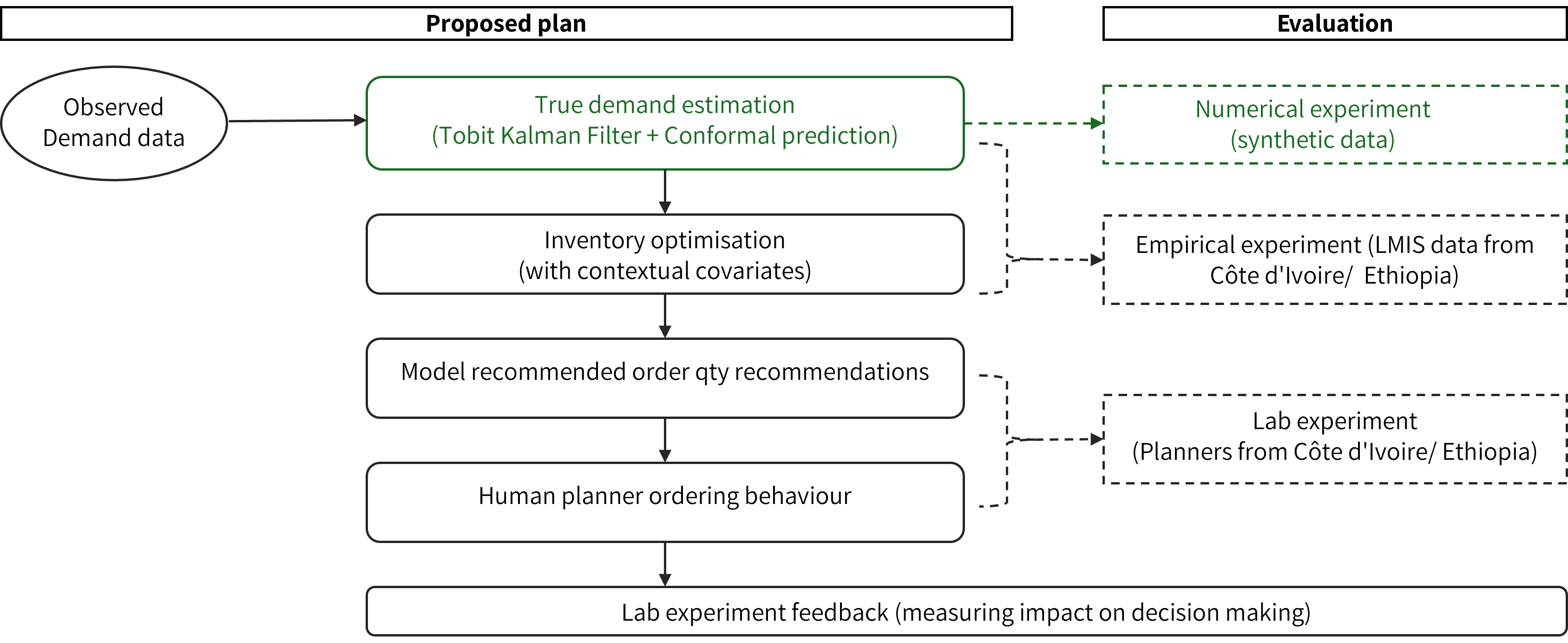
First stage: estimating true demand under censorship using tobit kalman filtering and conformal prediction

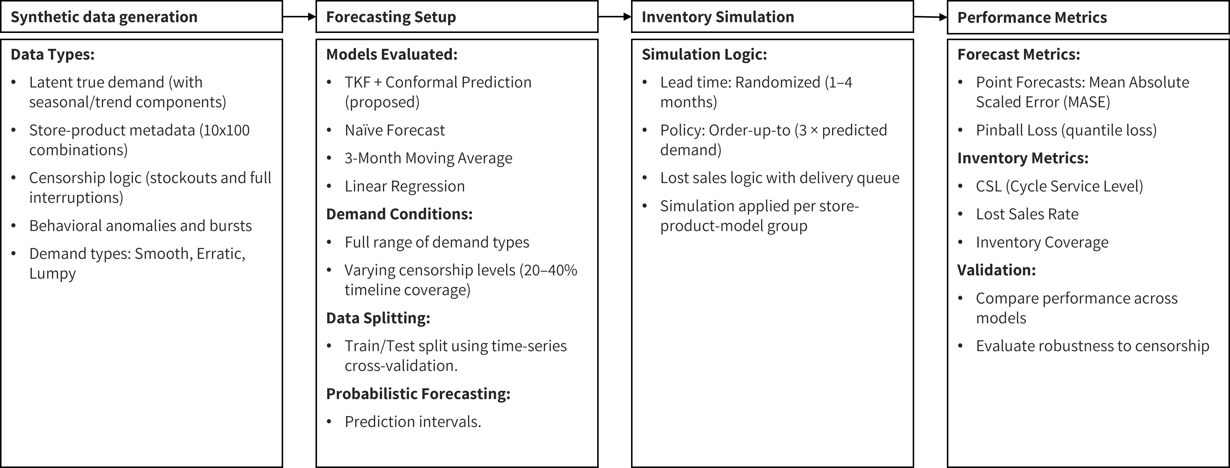
Experiment setup
Data exploration
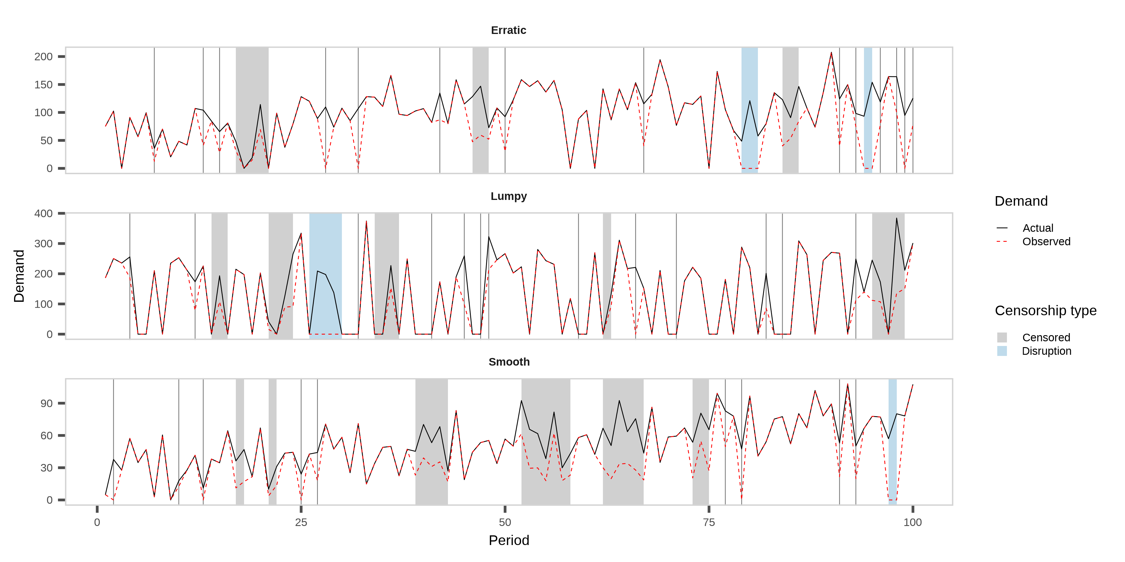
Actual vs. observed demand for one representative series per type × category, with disruptions and censoring shaded.
Actual vs forecasted demand distributions
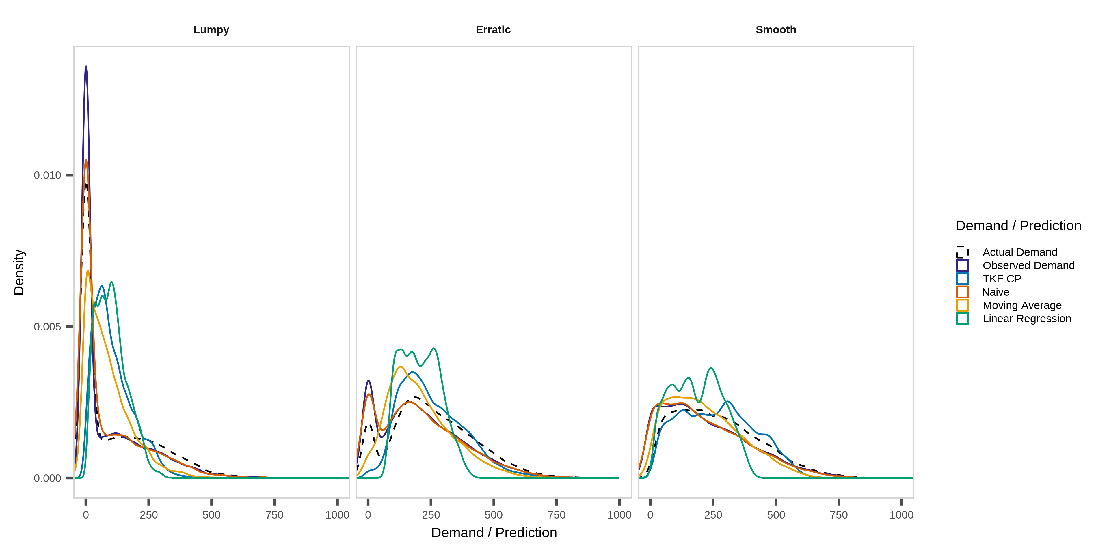
Figure 2: Actual vs. forecasted demand distributions for the different forecasting methods.
Performance evaluation - Nemenyi test
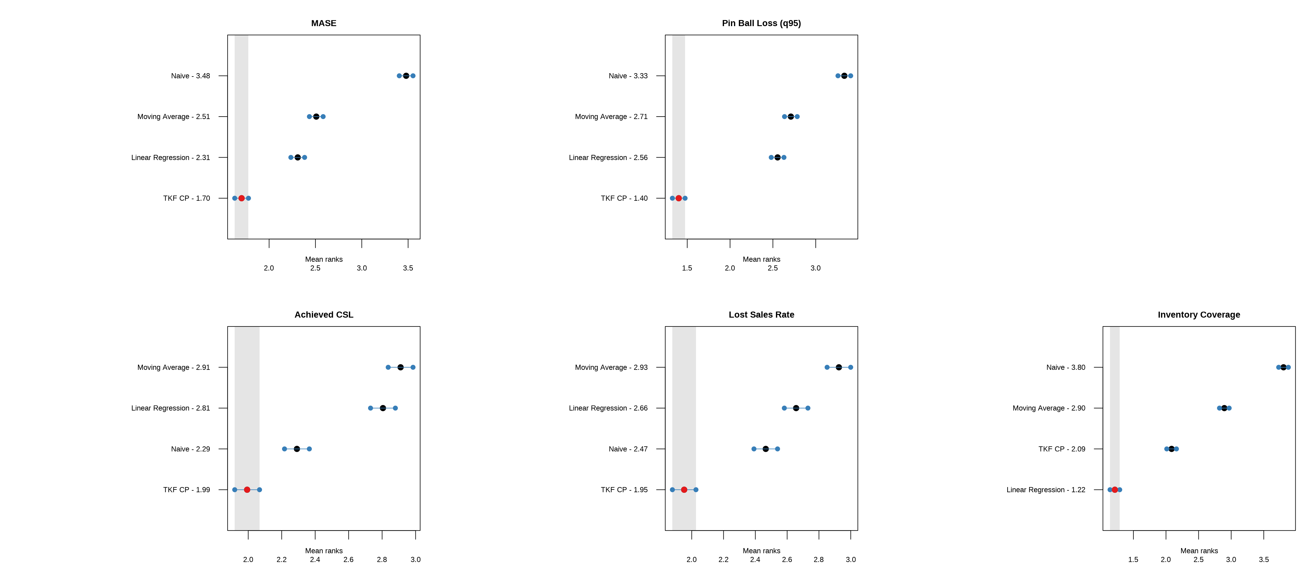
Figure 3: Average ranks of forecasting methods with 95% confidence intervals based on the Nemenyi test for all metrics. Lower ranks indicate better performance.
Performance evaluation - forecasting

Figure 4: Forecasting metrics for each series type for the different forecasting methods.
Performance evaluation - inventory

Figure 5: Inentory metrics for each series type for the different forecasting methods.
Way forward

Develop a more comprehensive inventory policy using forecasted quantiles → Incorporate uncertainty directly into order decisions
Extend empirical model with external covariates → Account for special events, disruptions, and policy shifts
Conduct lab experiment with real demand planners → Measure how model recommendations affect decision-making
Materials

You can find the slides here.