![]()
![]()


Outline

What was never COUNTED . . .
The fundamental question
What we are going to do
Numerical experiment
What’s NEXT
Seen the UNSEEN
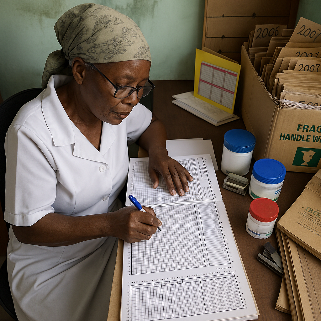
Human story: What data misses

Nilu went to a pharmacy for Product A.
It was not in stock and the system logs it as
zero demand.
This creates broken trust and leads to create
UNMET DEMAND.
Seen the UNSEEN
Analytical reality: Why this matters

Stockouts censor demand.
Observed sales ≠ actual demand.
Inventory decisions based on this false signal?
Understocking → more stockouts.
Forecasts don’t just underperform. They miss the whole story.
A lost sale = a lost opportunity for care.
Contraceptive products aren’t easily SUBSTITUTED
The BIG PICTURE

In reality…
There are more than
218 million women
like Nilu still have an unmet need for family planning.
Ultimately, this results in dropouts, unwanted pregnancies, and almost 7 million hospitalizations each year in developing countries.
Why this is critical
- Frequent stockouts are common in family planning supply chains, especially in developing countries, significantly impacting public health outcomes.
- During my recent field visit to Ethiopia, stockouts were repeatedly identified by demand planners as a major barrier to effective contraceptive supply management.
- Traditional forecasting methods fail under censorship.
- Prior research inadequately addresses demand estimation under conditions of frequent stockouts and interruptions, often leading to biased forecasts and suboptimal inventory decisions.
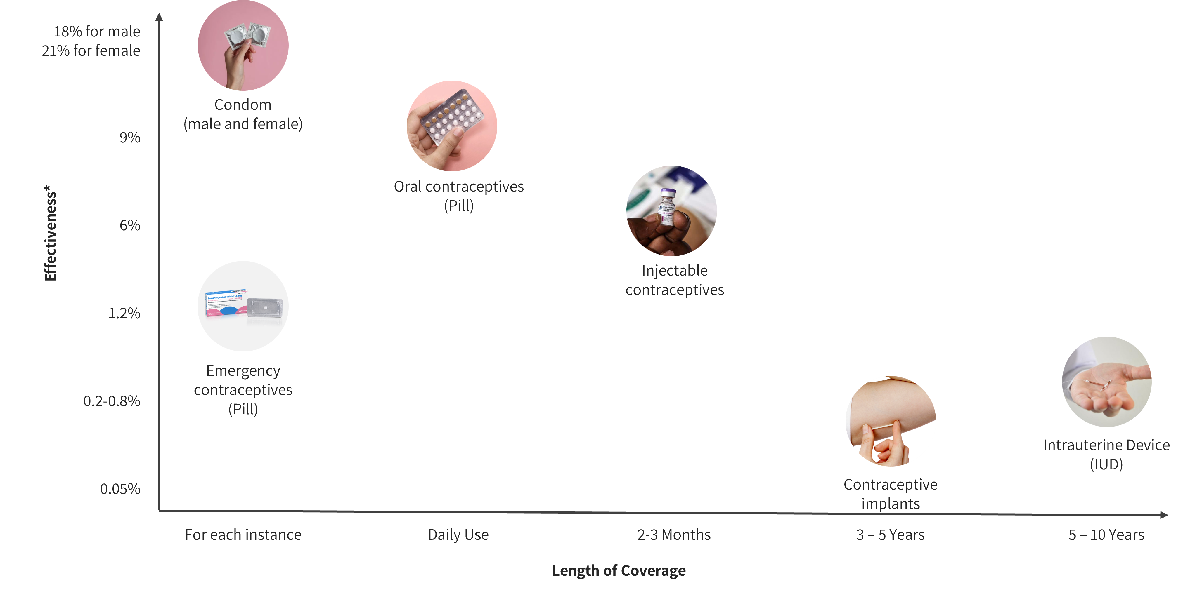
Censorship scenarios
How can a demand forecasting and inventory optimization model that incorporates lost sales estimation and contextual field data enhance contraceptive supply chain performance and reduce stockouts in developing countries?
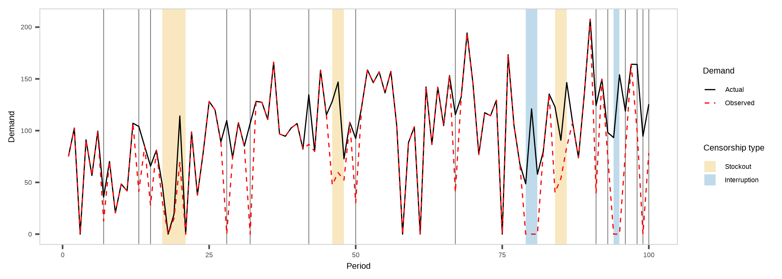
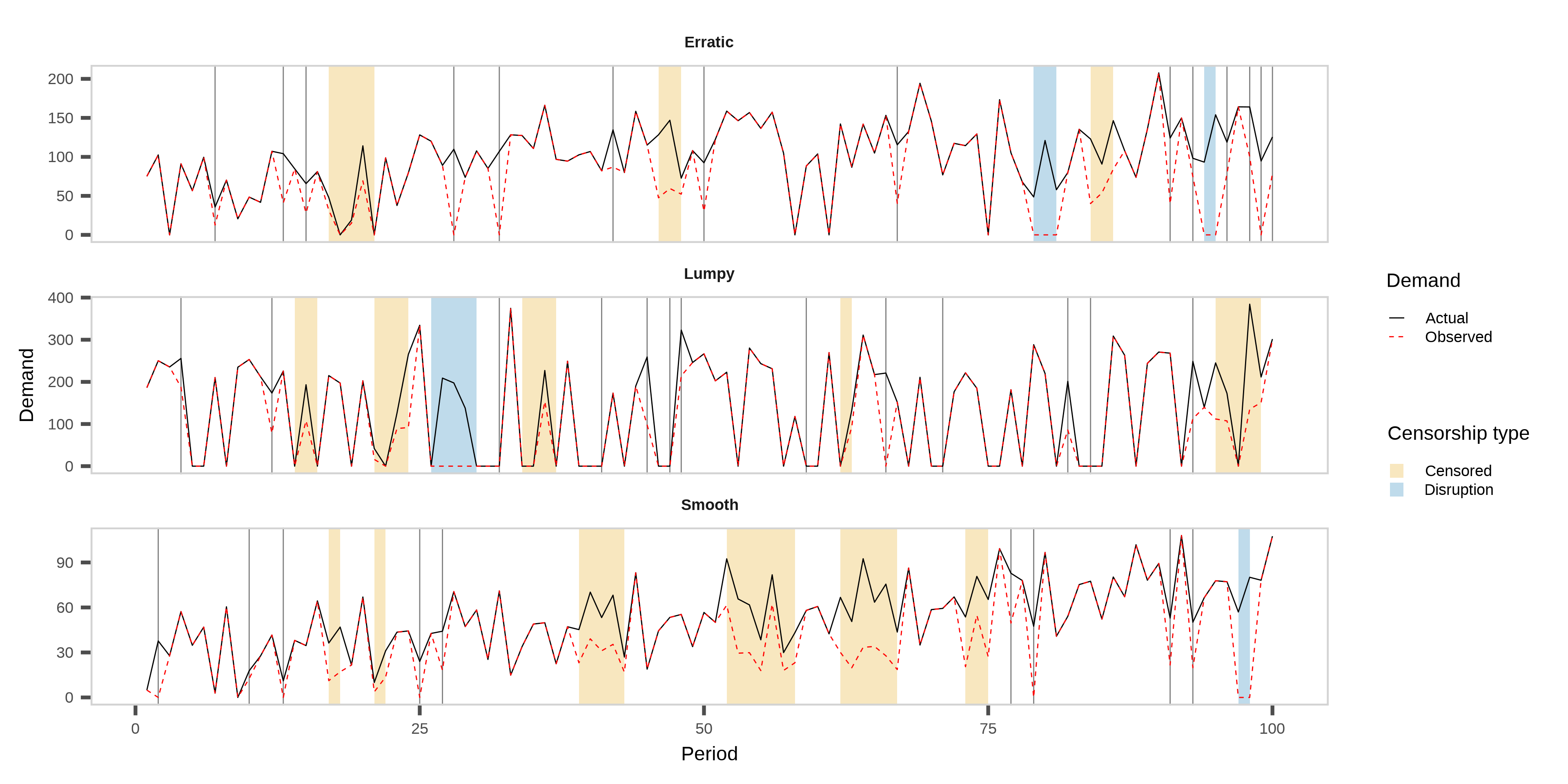
Figure 1: Censorship scenarios in family planning supply chains.
How we can fill the gaps

- RQ1: How accurately can a Tobit Kalman Filter with conformal prediction estimate true demand under censorship?
- RQ2: How does demand reconstruction improve inventory performance compared to baseline planning methods?
- RQ3: How do planners adjust their orders in response to proposed model-generated recommendations?
Our proposed framework

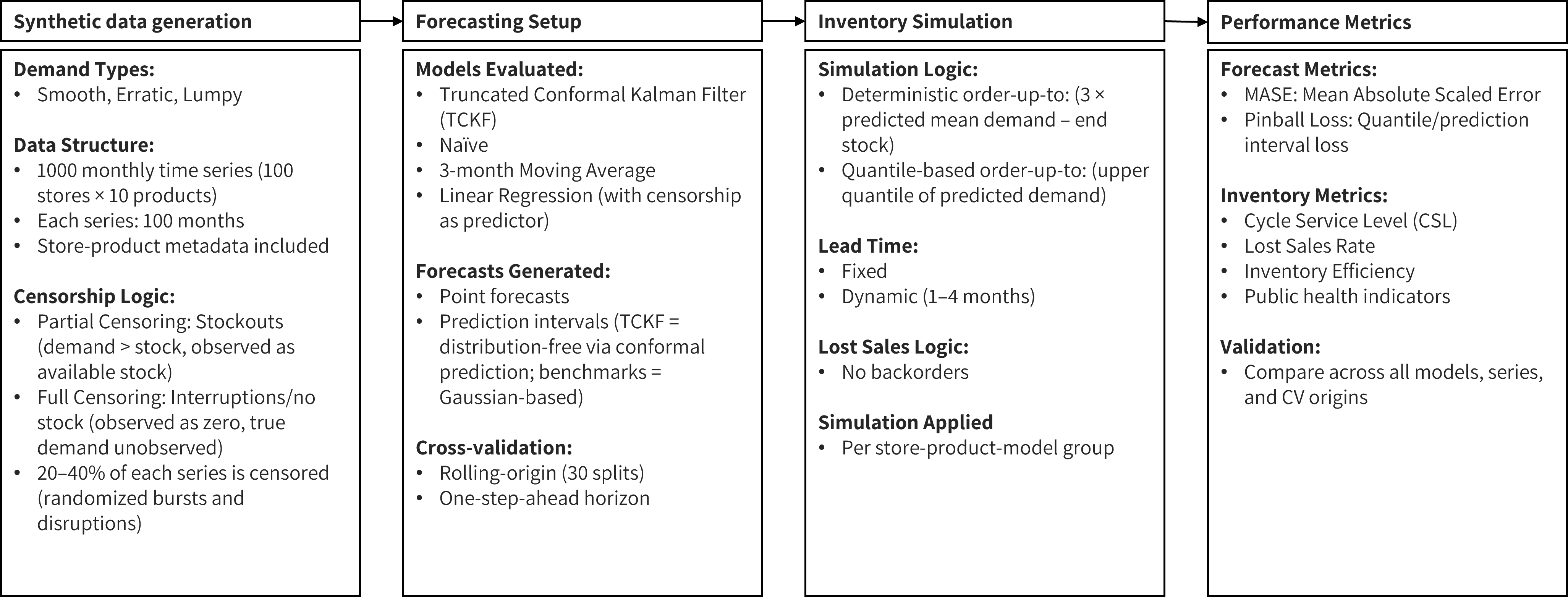
Experiment setup
Synthetic data exploration - example

Actual vs. observed demand for one representative series per type, with disruptions and censoring shaded.
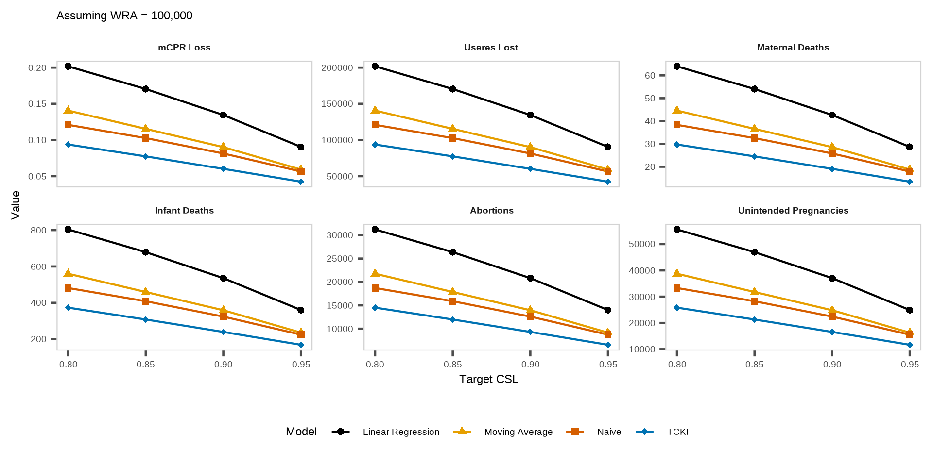
Overall forecasting and inventory performance across models
Policy 2: quantile-based order-up-to level (uncertainty-aware target) - 1 month leadtime
Public healthcare indicators across models
Policy 2: quantile-based order-up-to level (uncertainty-aware target) - 1 month leadtime
Way forward

Add more benchmarking methods → e.g., Censored ETS,...
Extend empirical model with external covariates → Account for special events, disruptions, and policy shifts
Conduct a lab experiment with real demand planners → Measure how model recommendations affect decision-making
Any questions or thoughts? 💬