Cardiff University

Data Lab for Social Good

ukri

wgsss

usaid


WHAT WAS LOST

Estimating censored demand in family planning supply chains with the Truncated Conformal Kalman Filter


Harsha Halgamuwe Hewage
Data Lab for Social Good Research Group, Cardiff University, UK

Lead Supervisor: Prof. Bahman Rostami-Tabar
Co Supervisors: Prof. Aris Syntetos & Dr. Federico Liberatore


2025-09-16

Outline


Outline graphic

What was never COUNTED . . .

The fundamental question

What we are going to do

Empirical evaluation

What NEXT?

WHAT WAS NEVER COUNTED…

Seen the UNSEEN

Human story: What data misses

Outline graphic

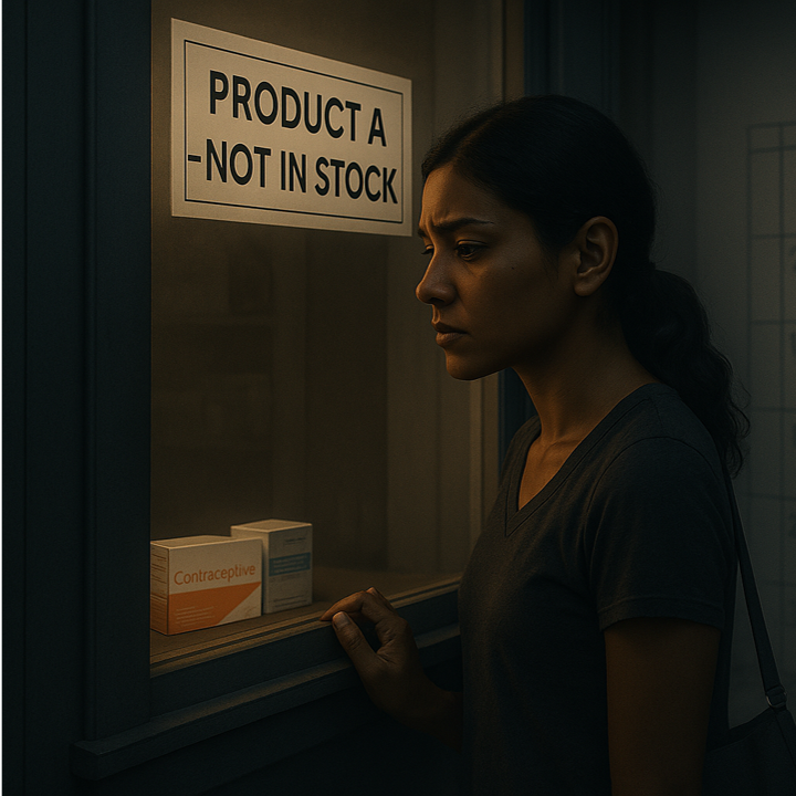
Nilu went to a pharmacy for Product A. It wasn’t in stock.


The system logs it as zero demand.


But the need was real. The system just missed it.


This creates broken trust and leads to create

UNMET DEMAND.

Seen the UNSEEN

Analytical reality: Why this matters

Outline graphic

In supply chains like this, Stockouts censor demand.

Observed sales ≠ actual demand.


Inventory decisions based on this false signal?
Understocking → more stockouts.


Forecasts don’t just underperform. They miss the whole story.


A lost sale = a lost opportunity for care.

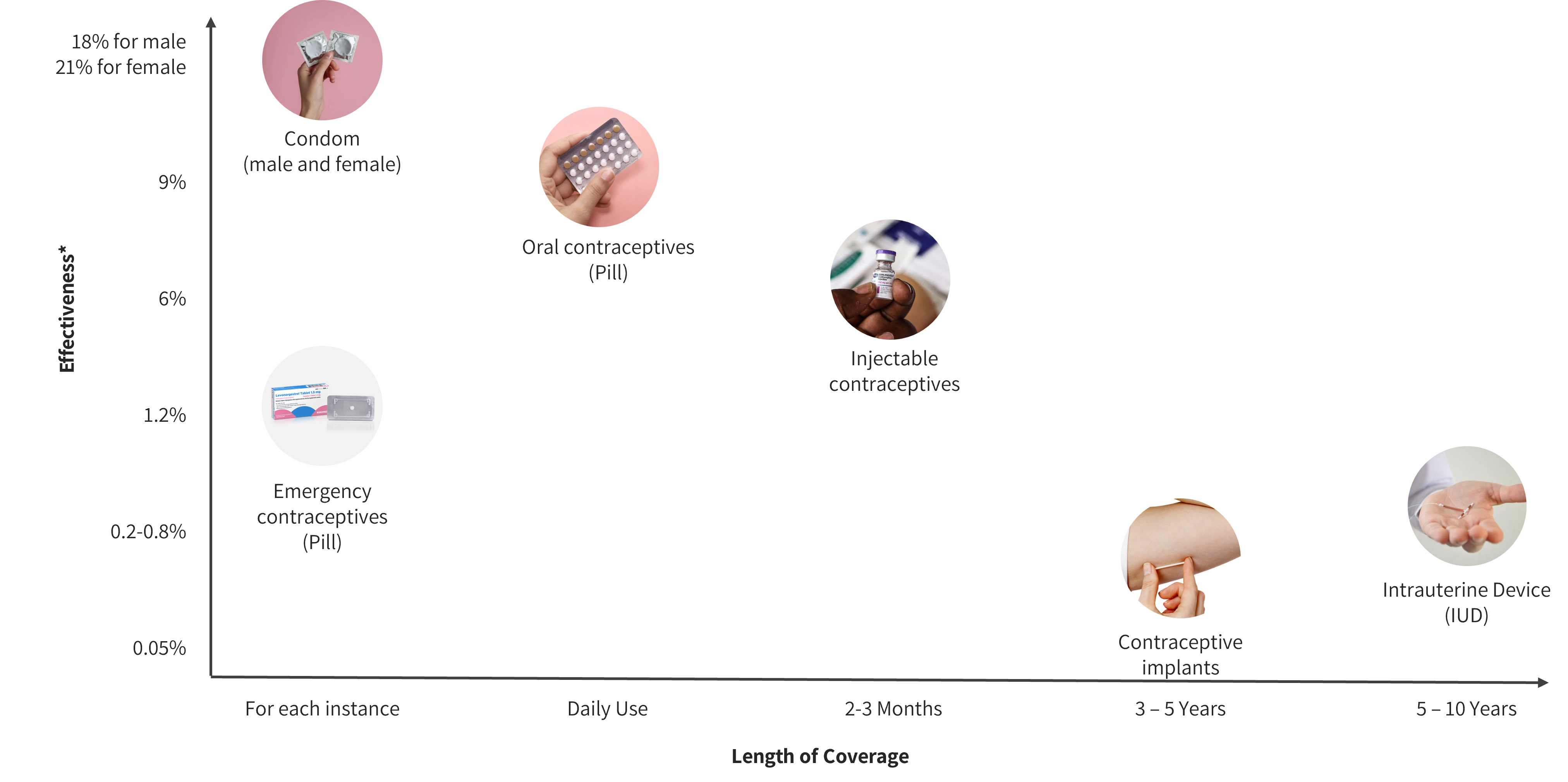
Contraceptive products aren’t easily SUBSTITUTED


Story panel

The BIG PICTURE


Story panel

In reality…

There are more than

218 million women

like Nilu still have an unmet need for family planning.

Ultimately, this results in dropouts, unwanted pregnancies, and almost 7 million hospitalizations each year in developing countries.

Why this is critical
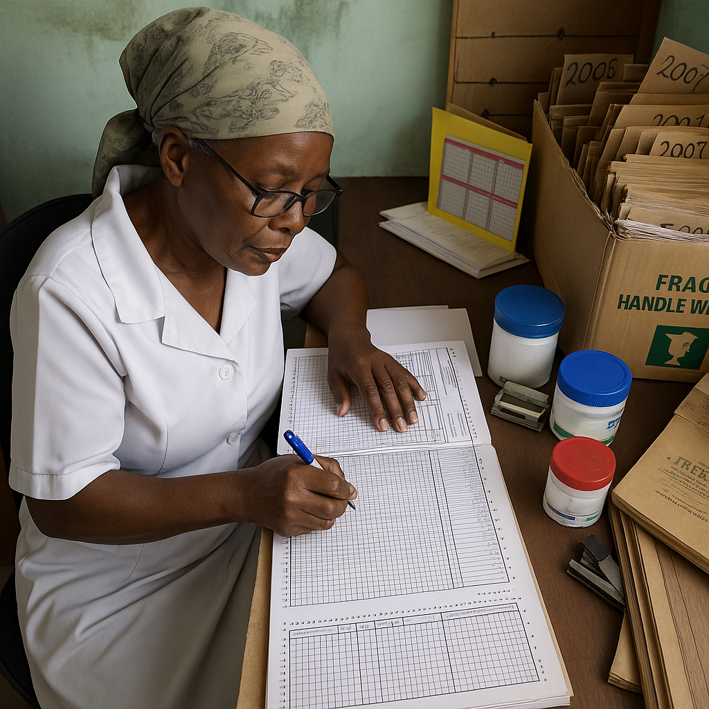

Story panel

  • Censorship is structural — stockouts and interruptions are common in FPSC, not rare events.
  • Field insight — in Côte d’Ivoire and Ethiopia, demand planners repeatedly flagged stockouts as the key barrier.
  • Forecasting fails under censorship — observed sales understate true demand.
  • The literature split - prior research often separates forecasting from inventory decisions.
  • Resources are tightening — with USAID withdrawal, high service levels must be achieved efficiently.

THE FUNDEMENTAL QUESTION

Key definitions


  • Stockouts: Periods when demand is higher than available inventory, leading to censored observations of demand.

  • Interruptions: Periods when no products are issued despite available stock, thus artificially recorded as zero demand.

  • Censored Demand: Demand occurring during periods when products are unavailable (stockouts or interruptions), thus not fully observable.

  • True Demand: Actual demand that would have occurred if sufficient stock was available or no service interruptions.

Bridging forecasting, inventory, and impact


How can a demand forecasting model that explicitly handles censored demand due to stockouts and service interruptions improve inventory performance and public health outcomes in contraceptive supply chains?

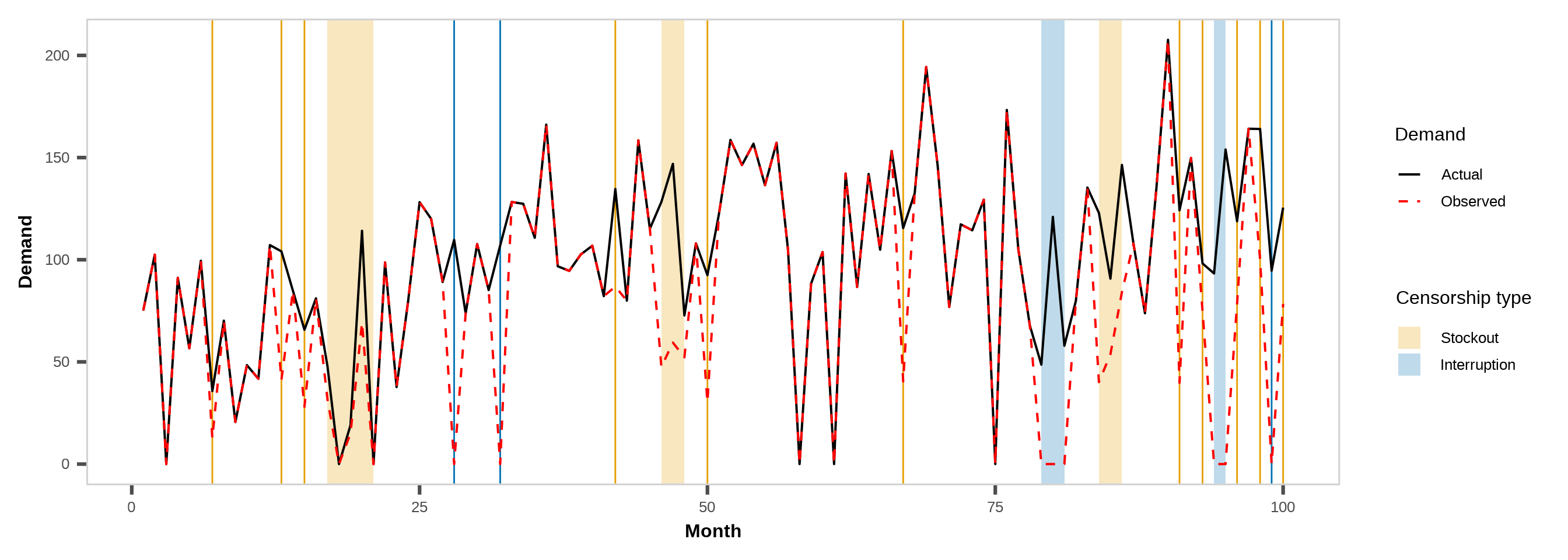
Figure 1: Censorship scenarios in family planning supply chains.

WHAT WE ARE GOING TO DO

How we can fill the gaps


Story panel

  • RQ1: How accurately can a Tobit Kalman Filter with conformal prediction estimate true demand under censorship?
  • RQ2: How does demand reconstruction improve inventory performance and healthcare impact compared to baseline planning methods?
  • RQ3: How do planner-adjusted forecasts compare to model-based methods in balancing availability and inventory efficiency?

Overview of the experimental framework


Truncated Conformal Kalman Filter (TCKF)

State-Space Formulation

\[ X_t = F X_{t-1} + \eta_t, \quad \eta_t \sim \mathcal{N}(0, Q_t) \]

  • \(X_t = [\ell_t, \tau_t, \gamma_t]^T\): level, trend, seasonality
  • \(F\): state transition matrix with seasonal decay and trend


Observation Equation with Censorship

\[ y_t = \begin{cases} H X_t + \nu_t & \text{if uncensored} \\ 0 & \text{if fully censored} \\ \min(H X_t, s_t) & \text{if partially censored} \end{cases} \]

  • \(H = [1, 0, 1]\): maps level and seasonality to observation
  • \(s_t\): stock available at time \(t\)


Kalman Prediction Step

\[ \mu_t = H \hat{X}_{t|t-1}, \quad \sigma_t^2 = H P_{t|t-1} H^T + R \]

Truncated Conformal Kalman Filter (TCKF)

Censored Observation Update

\[ \hat{y}_t = \mu_t + \sigma_t \cdot \frac{\phi(z_t)}{1 - \Phi(z_t)}, \quad z_t = \frac{y_t - \mu_t}{\sigma_t} \]

\[ \hat{X}_{t|t} = \hat{X}_{t|t-1} + K_t (\hat{y}_t - \mu_t) \]

  • Uses expectation of truncated Gaussian
  • For fully censored (\(y_t = 0\)), skip state update; propagate uncertainty


Conformal Prediction for Interval Estimation

\[ D_t \in [\max(0, \mu_t - q_\alpha), \mu_t + q_\alpha] \]

  • Residuals from uncensored periods used to calibrate \(q_\alpha\)
  • Ensures valid coverage without assuming normality


Note on Initialization: Initial state vector \(X_0 = [\ell_0, \tau_0, \gamma_0]^T\) is extracted via STL decomposition from uncensored periods.

Performance evaluation - Forecast

Point predictions

\[ Forecast\ Value\ Added = (1 -Rel\ RMSE) \times 100\% \] Values above 1 indicate better performance than TCKF.

\[ Rel\ RMSE = \frac{RMSE_{\text{Method}}}{RMSE_{\text{TCKF}}} \]

\[ RMSE = \sqrt{\frac{1}{n} \sum_{t=1}^{n} (\hat{y}_t - y_t)^2} \]

Probabilistic predictions

The pinball loss at time \(t\) for quantile level \(p\) is defined as:

\[ Q_{p,t} = \begin{cases} 2(1 - p)(\hat{f}_{p,t} - y_t), & \text{if } y_t < \hat{f}_{p,t} \\ 2p(y_t - \hat{f}_{p,t}), & \text{if } y_t \geq \hat{f}_{p,t} \end{cases} \]


\[ \text{Skill Score} = \frac{\text{Pinball Score}_{\text{TCKF}} - \text{Pinball Score}_{\text{Method}}}{\text{Pinball Score}_{\text{TCKF}}} \times 100\% \]

Values above 1 indicate better performance than TCKF.

Performance evaluation - Inventory


Cycle Service Level (CSL): proportion of periods in which stock was available

\[ CSL = \frac{1}{N} \sum_{t=1}^{N} \mathbb{1}(in\_stock_t = 1) \]

Stock-Out Rate (SOR): proportion of periods experiencing a stockout

\[ SOR = \frac{1}{N} \sum_{t=1}^{N} \mathbb{1}(stockout\_ev_t = 1) \]

Inventory Turnover (IT): average stock relative to the target level

\[ IT = \frac{1}{N} \sum_{t=1}^{N} \frac{average\_stock_t}{target\_stock_t}, \quad \text{if } target\_stock_t > 0 \]

Performance evaluation - Inventory

Relative CSL (Rel CSL):

\[ Rel\ CSL = \begin{cases} \frac{CSL - CSL_{TCKF}}{CSL_{TCKF}}, & CSL_{TCKF} \ne 0 \\ CSL - CSL_{TCKF}, & \text{otherwise} \end{cases} \]

Relative SOR (Rel SOR):

\[ Rel\ SOR = \begin{cases} \frac{SOR_{TCKF} - SOR}{SOR_{TCKF}}, & SOR_{TCKF} > 0 \\ 0, & SOR_{TCKF} = 0 \land SOR = 0 \\ -SOR, & SOR_{TCKF} = 0 \land SOR > 0 \end{cases} \]

Relative IT (Rel IT):

Let \(\Delta = |IT_{TCKF} - 1|\), then:

\[ Rel\ IT = \begin{cases} 0, & IT = 0 \land IT_{TCKF} = 0 \\ IT - 1, & IT_{TCKF} = 1 \\ 1 - \frac{|IT - 1|}{\Delta}, & \text{otherwise} \end{cases} \]


The composite Inventory Value Added score aggregates these components:

\[ IVA = w_{CSL} \cdot Rel\ CSL + w_{SOR} \cdot Rel\ SOR + w_{IT} \cdot Rel\ IT \]

Values above 1 indicate better performance than TCKF.

Performance evaluation - Healthcare impact


Stockout of one product can decrease mCPR by 6.5% points

\[ \Delta mCPR = 0.065 \times M \times (\text{Stockout Rate}_{\text{method}} - \text{Stockout Rate}_{\text{TCKF}}) \]


\[ \text{Users Lost} = \Delta mCPR \times \text{WRA Population} \]

where \(\text{WRA Population}\) is the number of women of reproductive age, and \(M\) is the number of distinct products considered.


  • Maternal deaths averted: \(\frac{\text{Users Lost}}{3153}\)
  • Infant deaths averted: \(\frac{\text{Users Lost}}{251}\)
  • Abortions averted: \(\frac{\text{Users Lost}}{6.46}\)
  • Unintended pregnancies averted: \(\frac{\text{Users Lost}}{3.63}\)

WHAT DID WE FIND

Empirical evaluation


  • Data source: Monthly LMIS records from Côte d’Ivoire (Jan 2016–Dec 2019)

  • Scope: 507 site–product time series covering 9 contraceptive methods (male & female condoms, emergency contraception, oral pills, injectables, implants, IUDs)

  • Training window: January 2016 – December 2018

  • Test window: January 2019 – December 2019

  • Cross-validation: Rolling-origin evaluation—re-train each month on all prior data, forecast 1-month ahead across the test year

Empirical data exploration

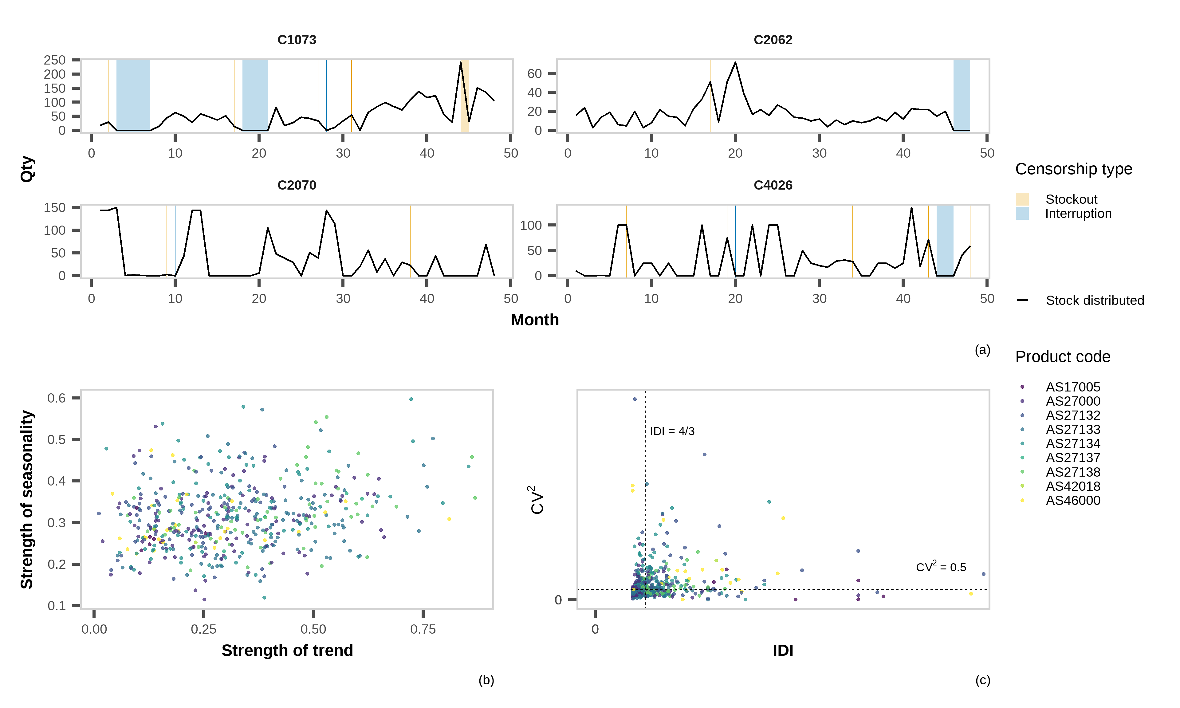
(a) Representative time series for each demand type; (b) Distribution of time series by trend and seasonality strength and; (c) Intermittency classification based on IDI and CV^2 thresholds.

Overall forecasting performance across models


Method Mean FVA Mean Skill Score (q80) Mean Skill Score (q85) Mean Skill Score (q90) Mean Skill Score (q95) Mean Skill Score (q97.5)
TCKF 0 0 0 0 0 0
ETS -0.86 -2.72 -2.67 -2.28 -2.05 -2.52
System Generated -0.97 -1.37 -1.69 -1.6 -1.81 -1.57
Mean -0.97 -2.73 -2.39 -2.38 -2.18 -2.26
TimeGPT -0.98 -4.05 -4.93 -6.84 -13.28 -20.99
Censored TimeGPT -1.01 -3.94 -4.71 -6.53 -12.79 -20.18
Censored Mean -1.02 -2.69 -2.38 -2.59 -2.4 -2.63
Syntetos-Boylan Approx -1.03 -2.74 -2.63 -3.22 -2.87 -3.16
ARIMA -1.19 -3.11 -3.05 -3.04 -3.06 -3.84
Censored ARIMA -1.19 -3.77 -3.45 -3.39 -3.28 -4.03
LightGBM -1.36 -3.39 -2.97 -2.93 -2.96 -3.14
Censored LightGBM -1.36 -3.54 -2.96 -2.93 -3.17 -3.42
Naive -1.7 -3.78 -3.43 -2.76 -2.85 -3.98
Censored Linear Regression -2.3 -3.95 -4.53 -5.8 -6.47 -7.52
Linear Regression -2.37 -3.55 -4.18 -5.12 -5.57 -6.88
Demand Planner -4.63 -13.53 -11.38 -9.11 -6.45 -5.01

Significance test - point forecast

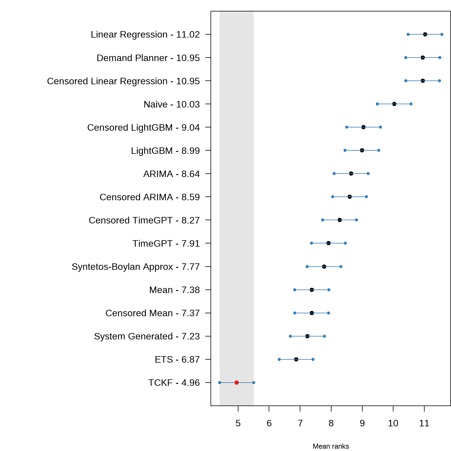
Figure 3: Nemenyi post-hoc test with 95% confidence level on inverted FVA values from the empirical evaluation.

Overall inventory performance

Existing mean based order-up-to level

Method Mean CSL Mean Stockout Rate Mean Inventory Turnover Mean IVA
Demand Planner 0.991 0.004 3.641 -2.931
LightGBM 0.966 0.034 1.271 -0.066
System Generated 0.955 0.023 4.048 -4.155
Censored LightGBM 0.95 0.041 1.652 -0.851
TCKF 0.929 0.055 1.087 0
Censored TimeGPT 0.927 0.061 1.516 -0.459
ETS 0.916 0.065 1.199 -0.191
TimeGPT 0.915 0.07 1.714 -0.855
Syntetos-Boylan Approx 0.913 0.077 1.003 -0.091
ARIMA 0.911 0.075 1.184 -0.256
Mean 0.896 0.078 1.507 -0.614
Linear Regression 0.892 0.083 1.878 -1.308
Censored Mean 0.891 0.082 1.236 -0.314
Censored Linear Regression 0.883 0.084 1.841 -1.267
Naive 0.877 0.072 2.423 -1.923
Censored ARIMA 0.876 0.106 1.041 -0.238

⚠️ High CSL often comes at the cost of overstocking

📉 Low inventory does not always equal efficiency

✅ TCKF achieves the most efficient trade-off

Overall inventory performance

Quantile based order-up-to level

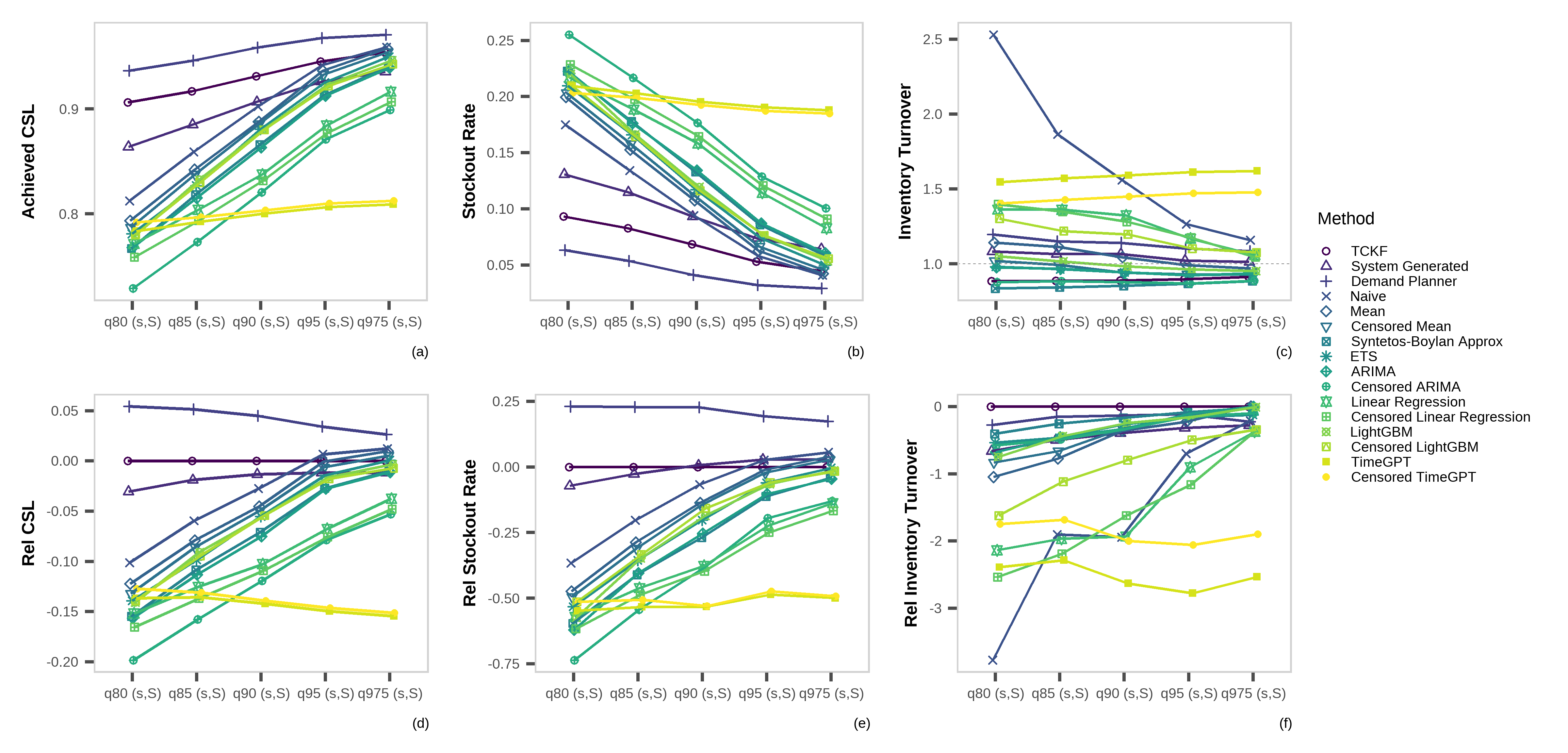
(a) Achieved CSL; (b) stockout rate; (c) inventory turnover; (d) relative CSL vs. TCKF; (e) relative stockout rate vs. TCKF; (f) relative inventory turnover vs. TCKF

Overall inventory performance

Quantile based order-up-to level

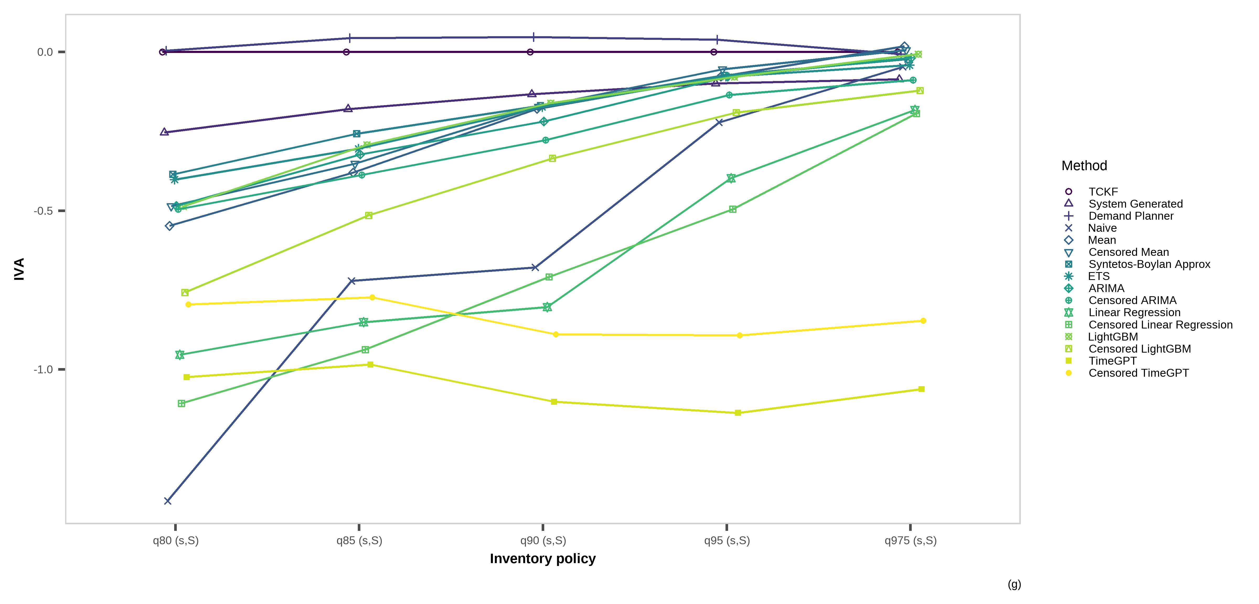
Figure 5: Inventory Value Added (IVA) vs. TCKF. under the quantile-based order-up-to level policy from the empirical evaluation.

Healthcare metrics

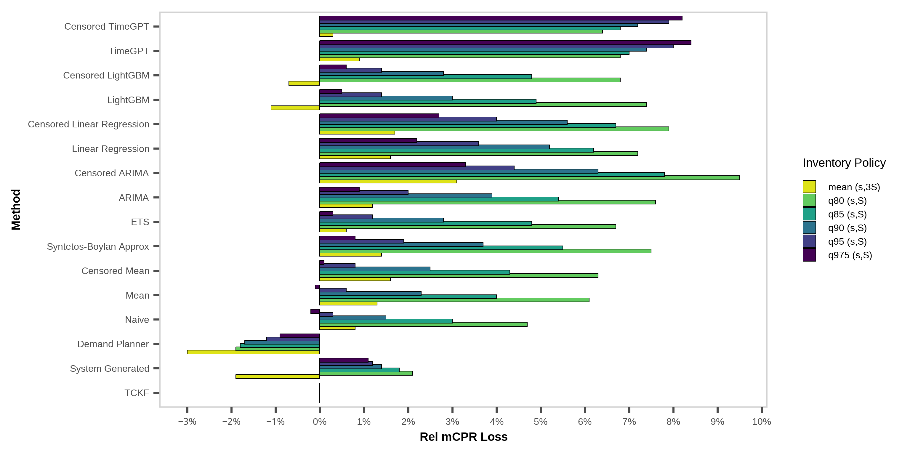
Figure 6: mCRP loss the empirical evaluation, based on relative stockout loss compared to the TCKF.

Illustrative impact: Why forecast quality matters


Outline graphic

In Côte d’Ivoire, ~1.59 million women use modern contraceptives (Track20).


Replacing TCKF with the current LMIS forecast under a q95 inventory policy would lead to:

🔻 reduce 18,599 additional women losing access

save 5,124 unintended pregnancies

save 5,879 abortions

save 54 infant deaths

WHAT NEXT

What matters: linking forecasts, inventory & health impact


Story panel

📌 Forecast accuracy ≠ forecast value

Most models focus on error metrics, but ignore censorship, uncertainty, and how forecasts are used.


📦 High service ≠ high performance

Demand Planner & System Forecast look strong, but hide poor forecasts behind excess inventory.


❤️ Forecast quality drives public health

Under lean policies (q80–q95), poor forecasts → more stockouts → more harm.

Key contributions & implications


Story panel

Addressing Censored Demand

TCKF explicitly accounts for stockouts and service interruptions by reconstructing true demand.

Forecasts Aligned with Inventory

Our study links forecasting with inventory decisions and public health outcomes.

Improved Inventory Efficiency

By reducing stockouts without overstocking, TCKF enhances both service levels and inventory turnover.

Practical Value for Planners & Donors

TCKF enables risk-aware, evidence-based planning — particularly valuable under resource constraints, such as the phasing out of USAID support.

Reproducibility & Extendability

The full pipeline is openly implemented in R using both synthetic and empirical LMIS data, supporting reproducibility.

Any questions or thoughts? 💬