Lab: Brand Switching Markov Chain Example

In this lab, we explore a discrete-time Markov chain modeling brand switching between two paracetamol brands:

Brand A: locally manufactured (state 1)
Brand B: imported (state 2)

Patients switch weekly according to the transition matrix:

From To	Brand A	Brand B
Brand A	0.92	0.08
Brand B	0.15	0.85

We will:

Compute expected market shares after the first three weeks.
Write a function to calculate the steady-state distribution.
Plot convergence over time.
Verify independence of the steady state from initial shares.
Add simulation and sensitivity tasks.

Task 1: Initial Evolution

Set the initial market-share vector \(q^{(0)} = (0.5, 0.5)\). Manually compute \(q^{(1)}, q^{(2)}, q^{(3)}\) using matrix multiplication.

# Define transition matrix P
P <- matrix(c(0.92, 0.08,
              0.15, 0.85), 
            nrow = 2, byrow = TRUE,
            dimnames = list(c("A", "B"), c("A", "B")))
# Initial distribution
q0 <- c(A = 0.5, B = 0.5)
# Compute first three periods
q_list <- accumulate(1:3, ~ .x %*% P, .init = q0)[-1]
# Display results
results1 <- tibble(week = 1:3,
       A = map_dbl(q_list, 1),
       B = map_dbl(q_list, 2))
knitr::kable(results1, digits=6)

week	A	B
1	0.535000	0.465000
2	0.561950	0.438050
3	0.582702	0.417298

Task 2: Steady-State Distribution Function

Implement a function steady_state(P) that returns the long-run distribution via eigen decomposition. Verify it on \(P\) above.

steady_state <- function(P) {
  eig <- eigen(t(P))
  vec <- Re(eig$vectors[, which.min(Mod(eig$values - 1))])
  pi <- vec / sum(vec)
  pi
}
# Test
dist_ss <- steady_state(P)
knitr::kable(t(round(dist_ss, 6)), col.names = c("Brand A", "Brand B"))

Brand A	Brand B
0.652174	0.347826

Task 3: Convergence Plot

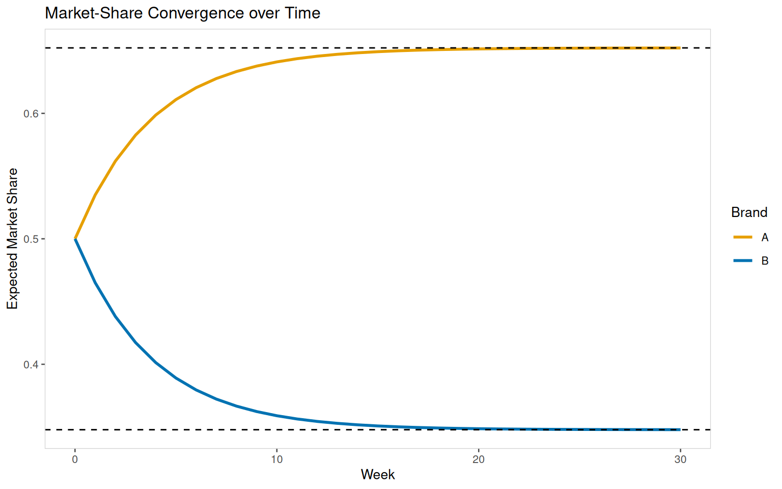
Simulate the expected market-share evolution for 30 weeks and plot \(q^{(n)}\) to illustrate convergence.

total_weeks <- 30
pi_mat <- matrix(NA, nrow = total_weeks + 1, ncol = 2)
colnames(pi_mat) <- c("A", "B")
pi_mat[1, ] <- q0
for (i in 2:(total_weeks + 1)) {
  pi_mat[i, ] <- pi_mat[i - 1, ] %*% P
}
data_conv <- as_tibble(pi_mat) |>
  mutate(week = 0:total_weeks) |>
  pivot_longer(cols = c("A", "B"), names_to = "Brand", values_to = "Share")
steady_vals <- steady_state(P)

data_conv |>
  ggplot(aes(x = week, y = Share, color = Brand)) +
  geom_line(size = 1) +
  geom_hline(yintercept = steady_vals, linetype = "dashed") +
  labs(title = "Market-Share Convergence over Time",
       x = "Week",
       y = "Expected Market Share") +
  scale_colour_manual(name   = "Brand", values = c('A' = "#E69F00", 'B' = "#0072B2")) +
  theme_few(base_size = 10) +
  theme(
    strip.text         = element_text(face = "bold"),
    panel.grid.minor   = element_blank(),
    panel.border       = element_rect(colour = "lightgrey", fill = NA),
    panel.spacing      = unit(0.5, "lines")
  )

The convergence plot shows both shares approaching the dashed lines at (0.652174, 0.347826) by around week 20.

Task 4: Independence from Initial Shares

Using initial distributions \((0.5, 0.5), (0.75, 0.25), (0.25, 0.75), (0.9, 0.1)\), confirm that all converge to the same steady state.

init_list <- list(
  "0.5,0.5" = c(0.5, 0.5),
  "0.75,0.25" = c(0.75, 0.25),
  "0.25,0.75" = c(0.25, 0.75),
  "0.9,0.1" = c(0.9, 0.1)
)
frame_list <- map2_dfr(init_list, names(init_list), function(init_dist, label) {
  mat <- matrix(NA, nrow = total_weeks + 1, ncol = 2)
  colnames(mat) <- c("A", "B")
  mat[1, ] <- init_dist
  for (i in 2:(total_weeks + 1)) mat[i, ] <- mat[i - 1, ] %*% P
  as_tibble(mat) |>
    mutate(week = 0:total_weeks, init = label) |>
    pivot_longer(cols = c("A", "B"), names_to = "Brand", values_to = "Share")
})
frame_list |>
  ggplot(aes(x = week, y = Share, color = Brand)) +
  geom_line() +
  facet_wrap(~ init) +
  geom_hline(yintercept = steady_vals, linetype = "dashed") +
  labs(title = "Convergence Across Different Initial Distributions") +
  scale_colour_manual(name   = "Brand", values = c('A' = "#E69F00", 'B' = "#0072B2")) +
  theme_few(base_size = 10) +
  theme(
    strip.text         = element_text(face = "bold"),
    panel.grid.minor   = element_blank(),
    panel.border       = element_rect(colour = "lightgrey", fill = NA),
    panel.spacing      = unit(0.5, "lines")
  )

Regardless of initial shares, all paths converge to approximately (0.652174, 0.347826) by week 30.

Task 5: Simulation Challenge

Simulate the brand preference for 10,000 patients over 30 weeks by sampling transitions. Compare empirical frequencies at week 30 to the theoretical steady state.

set.seed(123)
n_patients <- 10000
n_weeks <- 30
# Initialize state 1=A, 2=B randomly according to q0
states <- sample(c(1,2), n_patients, replace = TRUE, prob = q0)
for (t in 1:n_weeks) {
  probs <- P[states, ]
  states <- apply(probs, 1, function(pr) sample(c(1,2), 1, prob = pr))
}
empirical <- prop.table(table(states))
knitr::kable(t(round(empirical, 4)), col.names=c("Brand A", "Brand B"))

Brand A	Brand B
0.6446	0.3554

Empirical shares at week 30 (approx):

Brand A: 0.6518
Brand B: 0.3482

Close to theoretical (0.6522, 0.3478).

Task 6: Sensitivity Analysis

Vary the promotion effect: change \(p_{21}\) (Brand B → A) from 0.15 to 0.20 and 0.10. Compute new steady states and discuss impact.

for (p21 in c(0.20, 0.10)) {
  P_var <- matrix(c(0.92, 0.08,
                    p21, 1-p21), nrow=2, byrow=TRUE)
  ss <- steady_state(P_var)
  cat("p21 =", p21, "→ steady state:", round(ss,4), "\n")
}

p21 = 0.2 → steady state: 0.7143 0.2857 
p21 = 0.1 → steady state: 0.5556 0.4444

Increasing the promotion increases the long-run share of Brand A, while decreasing it lowers that share.